This page is devoted to the post-processing stage in SimpleMC. After adding a cosmological model, the user should first navigate to the SimpleMC directory and inspect the baseConfig.ini file. Here, the developer explains the different sampler options, dataset choices, and post-processing settings used throughout the analysis.
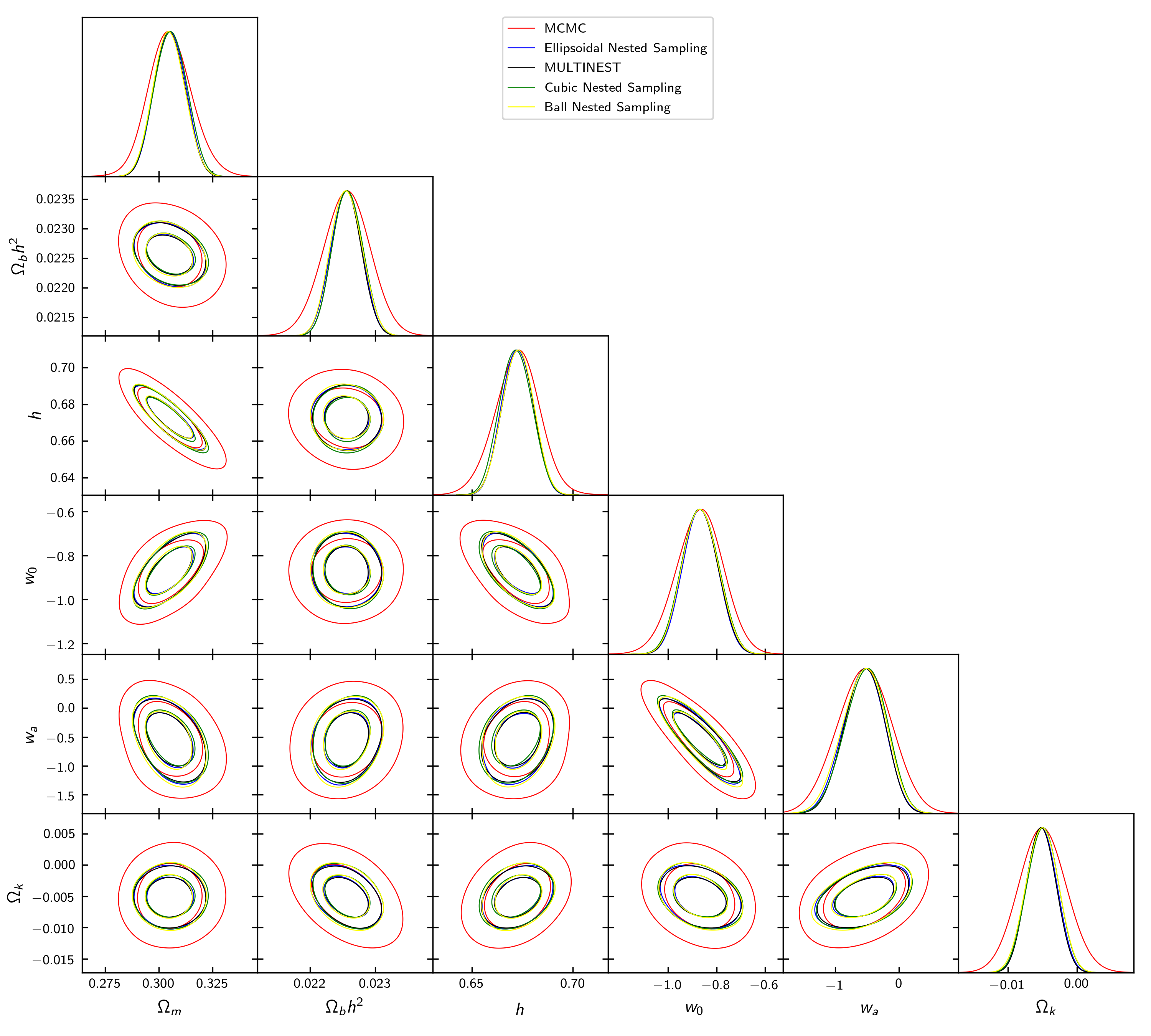
Now, we will continue our discussion by exploring the JBP model after adding it to SimpleMC. In this tutorial, I will use the nested sampling algorithm via the dynesty Python package with the multi bounding option. Before that, I also show an example where we use the dynesty Python package with the 'ellipsoidal', 'multinest', 'balls', and 'cubes' bounding options, together with the standard MCMC configuration options used in SimpleMC for cosmological analyses, as shown below.
1. Adding New .ini file SimpleMC
Now, I will explain how we can add a .ini file where you will define where the chains will be stored, the choice of the model, the choice of datasets, and the sampler settings. Below, you will find an example. You need to create your .ini file in the SimpleMC directory, let us say with the name jbp.ini.
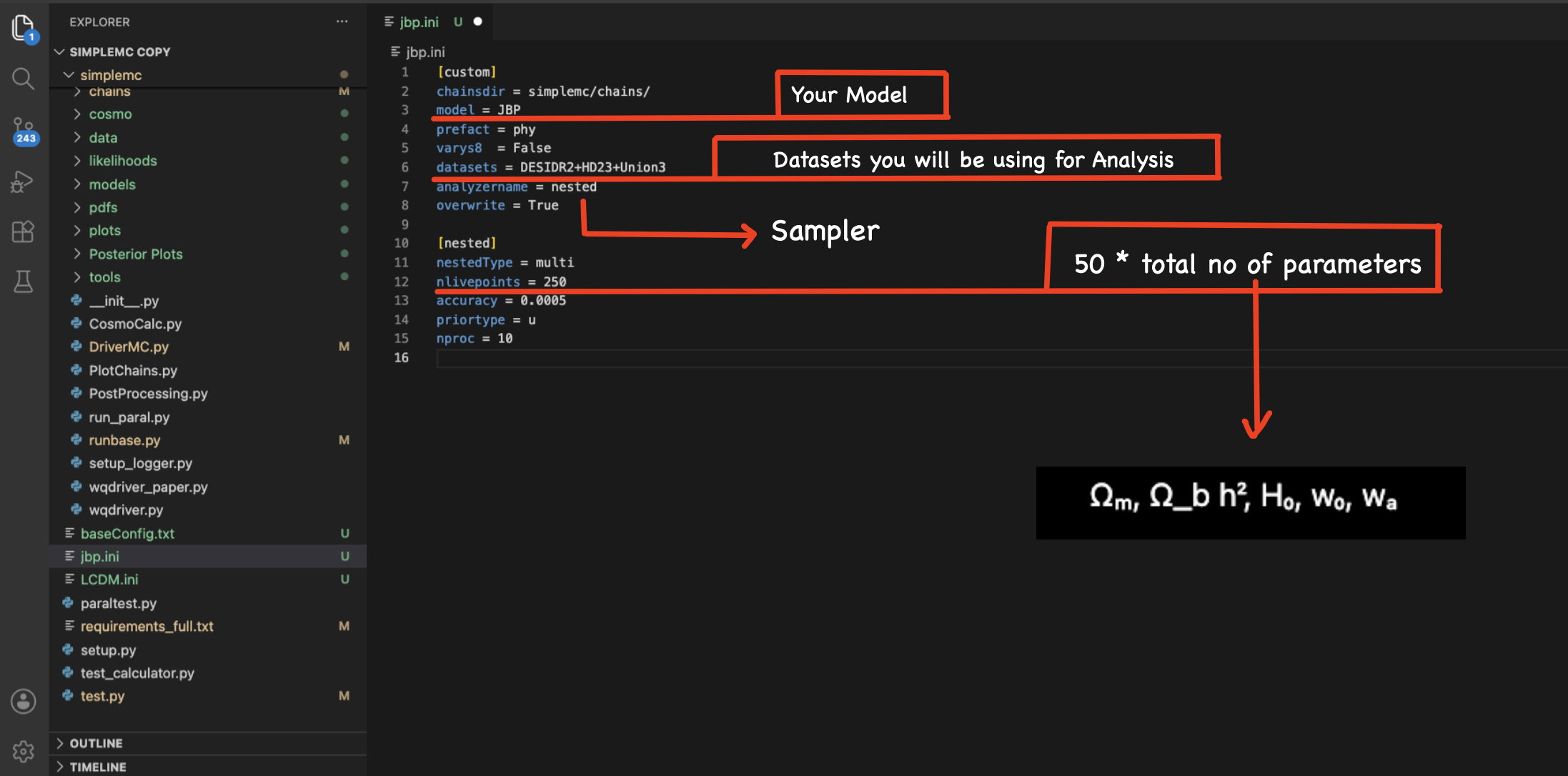
Find below the corresponding jbp.ini file.
[custom]
chainsdir = simplemc/chains/
model = JBP
prefact = phy
datasets = DESIDR2+HD23+Union3
analyzername = nested
overwrite = True

[nested]
nestedType = multi
nlivepoints = 250
accuracy = 0.0005
priortype = u
nproc = 10
2. Give your path in the test.py
Now, go to the SimpleMC directory and open the test.py file. Then, add the name of your corresponding .ini file, for example jbp.ini.
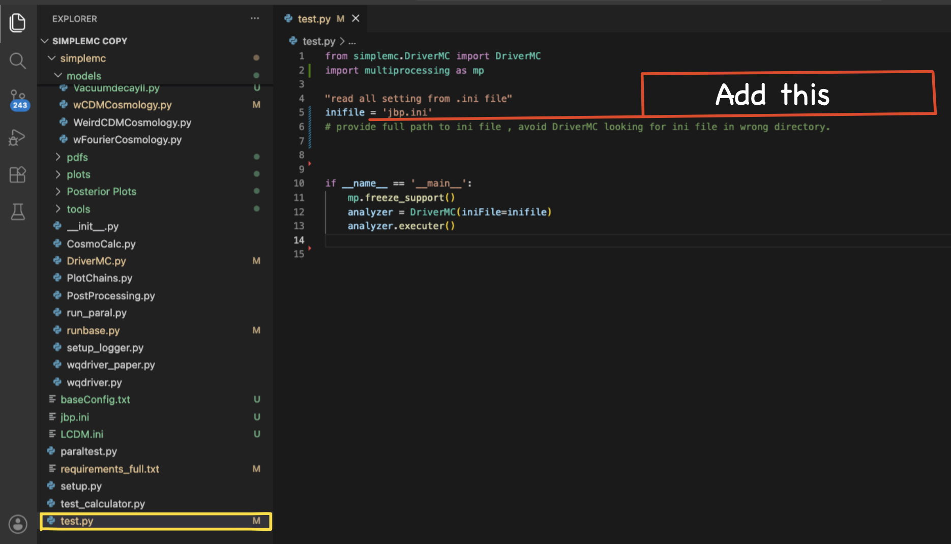
Find below the corresponding test.py file.
from simplemc.DriverMC import DriverMC
import multiprocessing as mp

"read all setting from .ini file"
inifile = "jbp.ini"

if __name__ == '__main__':
    mp.freeze_support()
    analyzer = DriverMC(iniFile=inifile)
    analyzer.executer()
Now, open your terminal, open the SimpleMC directory, activate the environment using conda activate simpleMC_env, and type python test.py to run the code.
Once the sampling process is completed, you will obtain several output files such as:
JBP_phy_DESIDR2+HD23+Union3_nested_multi_1.txtJBP_phy_DESIDR2+HD23+Union3_nested_multi_Summary.txtJBP_phy_DESIDR2+HD23+Union3_nested_multi.covmatJBP_phy_DESIDR2+HD23+Union3_nested_multi.maxlikeJBP_phy_DESIDR2+HD23+Union3_nested_multi.paramnames
Each of these files contains different information related to the analysis:
*_1.txt: contains the full chain samples generated during the nested sampling process, including parameter values, likelihoods, and weights.*_Summary.txt: provides a summary of the parameter constraints and statistical results.*.covmat: stores the covariance matrix of the sampled cosmological parameters.*.maxlike: contains the maximum-likelihood parameter values.*.paramnames: lists the parameter names and their corresponding LaTeX labels used in the analysis.
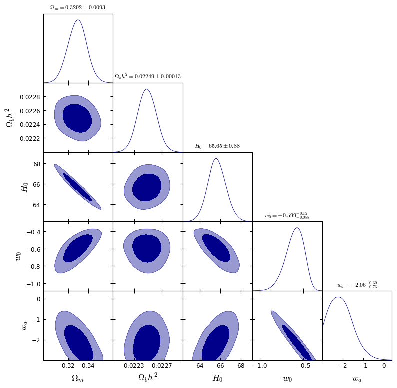
For post-processing and visualization, we are mainly interested in the file JBP_phy_DESIDR2+HD23+Union3_nested_multi_1.txt.
The following script reads the nested-sampling chain generated by SimpleMC, constructs the posterior samples with the appropriate weights, and uses GetDist to produce marginalized parameter constraints and triangle plots.
import numpy as np
from scipy.special import logsumexp
from getdist import MCSamples, plots
import matplotlib.pyplot as plt
import matplotlib as mpl
mpl.rcParams['mathtext.fontset'] = 'cm'

# ============================================================
# Load chain
# ============================================================
chain = np.loadtxt( "/path/to/your/chain/JBP_phy_DESIDR2+Planck_18+Union3_nested_multi_1.txt")

# ============================================================
# Nested weights
# ============================================================
logwt = chain[:,0]
negloglike = chain[:,1]
loglike = -negloglike

logwt_norm = logwt - logsumexp(logwt)
weights = np.exp(logwt_norm)

print("Sum of weights =", np.sum(weights))

# ============================================================
# Extract parameters
# ============================================================
Om   = chain[:,2]
Obh2 = chain[:,3]
h    = chain[:,4]
w0   = chain[:,5]
wa   = chain[:,6]

H0 = 100.0 * h

samples_array = np.vstack([Om, Obh2, H0, w0, wa,]).T

# ============================================================
# Create GetDist samples
# ============================================================
samples = MCSamples(samples=samples_array,weights=weights,loglikes=loglike,
    names=['Om','Obh2','H0','w0','wa'],
    labels=[r'\Omega_m', r'\Omega_b h^2', r'H_0', r'w_0', r'w_a',],ranges={'wa': (-3.0, None)})

# ============================================================
# Triangle Plot
# ============================================================
g = plots.getSubplotPlotter(width_inch=9)

g.settings.alpha_filled_add = 0.5
g.settings.axes_fontsize = 12
g.settings.lab_fontsize = 16
g.settings.legend_fontsize = 14

g.triangle_plot(samples, ['Om', 'Obh2', 'H0', 'w0', 'wa'], filled=True,
    contour_colors=['darkblue'],title_limit=1)

g.export("jbp.png")

plt.show()
3. Statistical Quantities and Model Comparison
After generating the posterior distributions and parameter constraints, we can move to the statistical quantities produced by the nested-sampling analysis.
The file *_Summary.txt contains a concise summary of the nested-sampling run and the resulting statistical quantities. A typical output looks like:
maxlike: 16.0822
logz: -33.0977 +/- 0.3429
where:
maxlikeis the maximum value of the likelihood found during the sampling process.logzis the natural logarithm of the Bayesian evidence (Z), together with its estimated uncertainty.
The Bayesian evidence is one of the key quantities produced by nested sampling and is defined as
\[Z=\int P(D\mid\theta,M)\,P(\theta\mid M)\,d\theta.\]where $P(D\mid\theta,M)$ is the likelihood of the observational data $D$ given the model $M$ and parameters $\theta$, and $P(\theta\mid M)$ is the prior probability distribution of the model parameters.
The value reported in the summary file as
logz: -33.0977 +/- 0.3429
This quantity corresponds to $\ln Z$, i.e., the Bayesian evidence expressed in logarithmic space. Since the evidence itself can span many orders of magnitude, it is customary to work with its logarithm when performing Bayesian model comparison.
Now, to compare the Bayesian evidence of two models for the same combination of observational datasets, one must first obtain the value of $\ln Z$ for the baseline model, which in our case is the $\Lambda$CDM model. Let model $i$ correspond to the JBP model and model $j$ correspond to the $\Lambda$CDM model. Now, to compare two cosmological models, one must compute the logarithmic Bayes factor,
\[\ln B_{ij} = \ln Z_i - \ln Z_j.\]For the same combination of observational datasets, we obtain for the $\Lambda$CDM model \(\ln Z_{\Lambda{\rm CDM}} = -33.8473 \pm 0.3805.\) Considering only the mean value of the Bayesian evidence, we use \(\ln Z_{\Lambda{\rm CDM}} = -33.8473.\) Similarly, for the JBP model, we obtain \(\ln Z_{\rm JBP} = -33.0977.\) We find \(\ln B_{ij} = \ln Z_{\rm JBP} - \ln Z_{\Lambda{\rm CDM}} = (-33.0977) - (-33.8473) = 0.7496.\)
The strength of evidence is commonly interpreted using the Jeffreys scale: $\ln B_{ij} < 1$ indicates inconclusive evidence, $1 \leq \ln B_{ij} < 2.5$ indicates weak evidence, $2.5 \leq \ln B_{ij} < 5$ corresponds to moderate evidence, $5 \leq \ln B_{ij} < 10$ indicates strong evidence, and $\ln B_{ij} \geq 10$ corresponds to decisive evidence in favor of model $i$ over model $j$. Conversely, if $\ln B_{ij}$ is negative, the preference is reversed and favors model $j$ over model $i$, with the strength of evidence interpreted according to the same Jeffreys scale using the magnitude of $\ln B_{ij}$.
Therefore, we obtain $\ln B_{ij}=0.7496$. According to the Jeffreys scale, this value corresponds to inconclusive evidence in favour of the JBP model over the $\Lambda$CDM model.
4. Covariance Matrix
SimpleMC also produces a covariance matrix file (*.covmat) containing the estimated parameter covariance matrix obtained from the posterior samples. The covariance matrix quantifies the uncertainties of the parameters as well as their correlations.
For the JBP model, a typical covariance matrix is stored as
JBP_phy_DESIDR2+HD23+Union3.covmat
The following script loads the covariance matrix and visualizes it as a correlation matrix:
import numpy as np
import matplotlib.pyplot as plt
import matplotlib as mpl

# ============================================================
# Matplotlib settings
# ============================================================
mpl.rcParams['mathtext.fontset'] = 'cm'
mpl.rcParams['font.size'] = 14

# ============================================================
# Load covariance matrix
# ============================================================
cov = np.loadtxt("/path/to/your/JBP_phy_DESIDR2+HD23+Union3.covmat", delimiter=",")

print("Covariance matrix shape:", cov.shape)
print(cov)

# ============================================================
# Parameter labels
# ============================================================
labels = [r'$\Omega_m$', r'$\Omega_b h^2$', r'$h$', r'$w_0$', r'$w_a$']

# ============================================================
# Convert covariance matrix to correlation matrix
# ============================================================
sigma = np.sqrt(np.diag(cov))
corr = cov / np.outer(sigma, sigma)

print("\nCorrelation matrix:")
print(corr)

# ============================================================
# Plot correlation matrix
# ============================================================
fig, ax = plt.subplots(figsize=(7, 6))
im = ax.imshow(corr, cmap='coolwarm', vmin=-1, vmax=1)

# Axis labels
ax.set_xticks(np.arange(len(labels)))
ax.set_yticks(np.arange(len(labels)))

ax.set_xticklabels(labels, fontsize=14, rotation=45, ha='right')
ax.set_yticklabels(labels, fontsize=14)

# Write correlation values inside cells
for i in range(corr.shape[0]):
    for j in range(corr.shape[1]):
        ax.text(
            j, i,
            f"{corr[i, j]:.2f}",
            ha='center',
            va='center',
            fontsize=11,
            color='black'
        )

# Colorbar
cbar = fig.colorbar(im, ax=ax, shrink=0.90,pad=0.04)
cbar.set_label('Correlation Coefficient', fontsize=14)
plt.tight_layout()

# Save figure
plt.savefig("JBP_correlation_matrix.png", dpi=300, bbox_inches='tight')
plt.show()
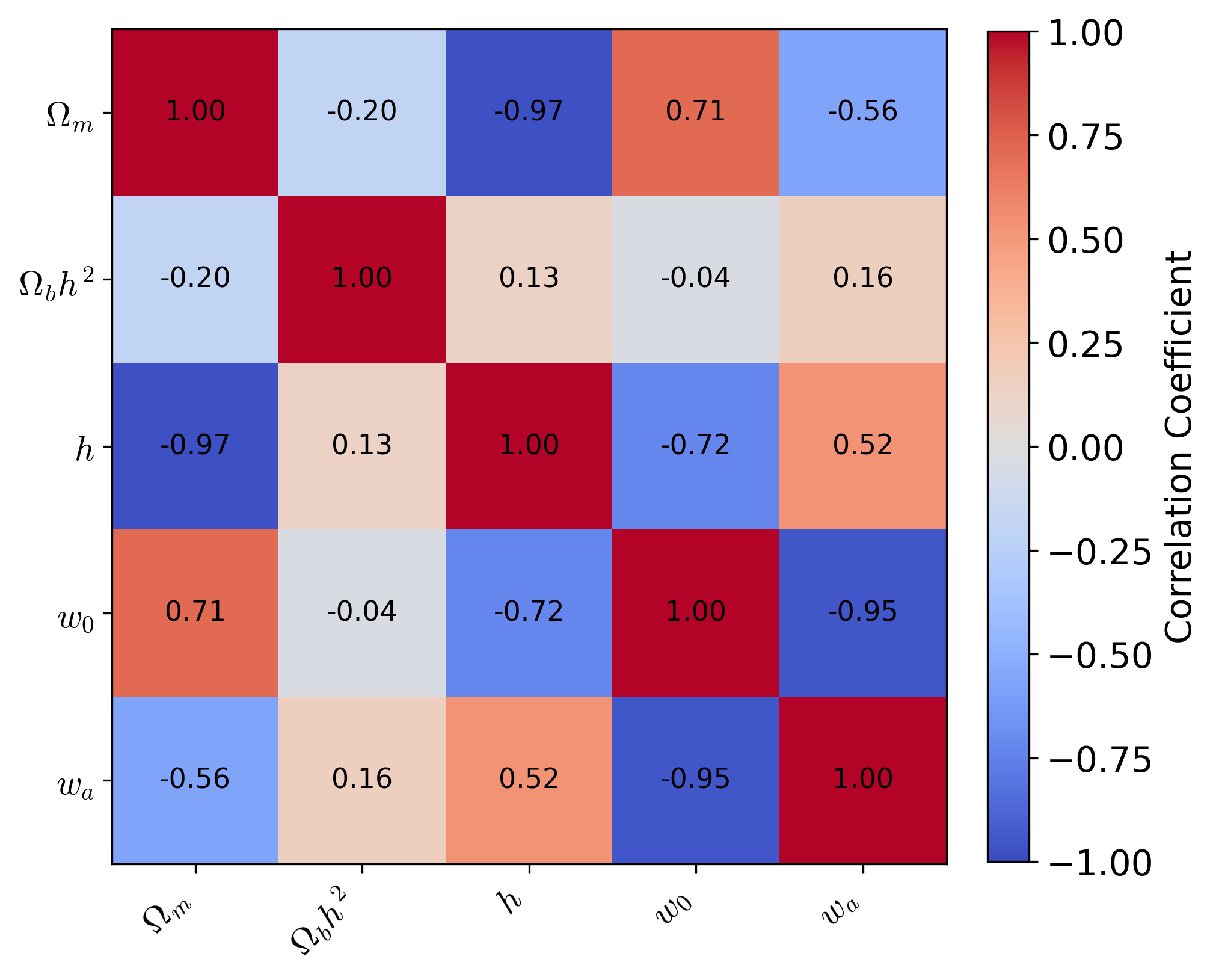
The diagonal elements of the covariance matrix correspond to the variances of the parameters, while the off-diagonal elements quantify correlations between different parameters. Positive values indicate correlated parameters, whereas negative values indicate anti-correlations. Converting the covariance matrix to a correlation matrix normalizes these quantities to the interval $[-1,1]$, making the parameter degeneracies easier to visualize and interpret.