This page is devoted to understanding the internal structure of SimpleMC and learning how to extend the code by implementing new cosmological models and likelihoods. In particular, we will focus on how to add a new dark energy parametrization within the SimpleMC framework and connect it with cosmological datasets through custom likelihood modules.
The diagram below is adapted from the original SimpleMC documentation by Isidro Gómez-Vargas and J. Alberto Vazquez.
Source: SimpleMC Structure Diagram
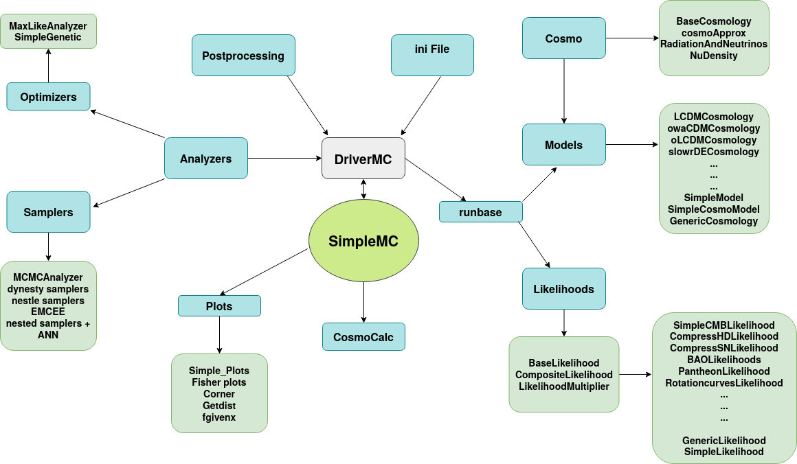
1. Structure of SimpleMC
The figure above shows the overall structure and workflow of SimpleMC. At the center of the framework is the DriverMC module, which acts as the main engine connecting cosmological models, likelihoods, samplers, optimizers, analyzers, and post-processing tools.
2. Main Components of SimpleMC
-
Cosmo This module contains the fundamental cosmological background quantities and basic cosmological calculations. Classes such as
BaseCosmology,RadiationAndNeutrinos, and related background modules are defined here. -
Models The
Modelsdirectory contains the cosmological models implemented inSimpleMC, such as:LCDMCosmologywCDMCosmologyowa0CDMCosmologyoLCDMCosmologyChaplyginCosmology, etc.
This is the main location where new dark energy parametrizations can be added.
-
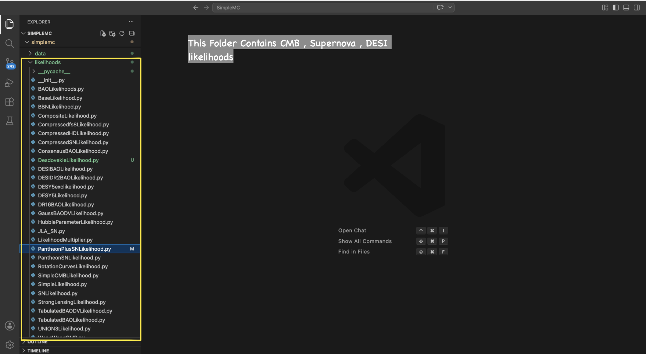
Likelihoods This module contains the observational likelihoods used for cosmological parameter estimation, including:
DESI DR2 BAO LikelihoodPantheonPlus Supernova LikelihoodCosmic Chronometer LikelihoodsCompressed CMB LikelihoodsRotation Curve LikelihoodsStrong Lensing Likelihoods, etc.
New likelihoods can also be implemented within this structure.
-
Samplers and Optimizers
SimpleMCsupports several Bayesian sampling and optimization algorithms, including:MCMC SamplersNested Sampling using the dynesty libraryMaximum Likelihood AnalyzerGenetic Algorithms (using the deap library)Particle Swarm Optimization (pyswarms)emcee, etc.
-
ini File and runbase The
.iniconfiguration files define the cosmological model, datasets, and sampler settings. Therunbasemodule connects these configurations to the internalSimpleMCpipeline.
3. Understanding the Structure of SimpleMC
Now, I will explain how to add a new dark energy model within SimpleMC. However, before doing that, we first need to understand the internal structure of SimpleMC and how the code is organized once you clone and install it. Below, you can see a schematic overview of the SimpleMC code.
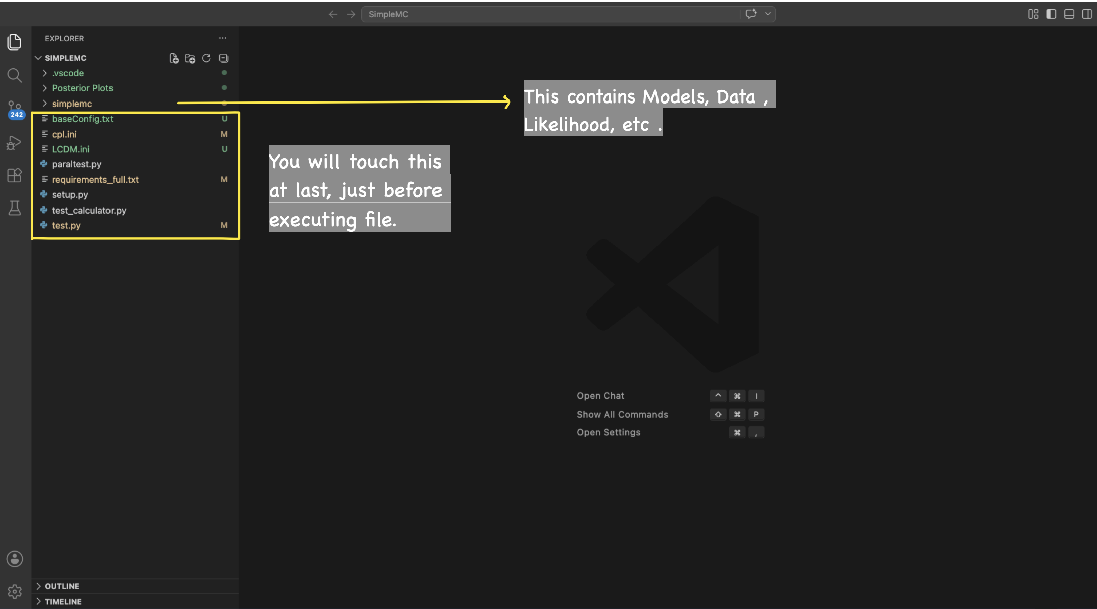
You will first find the parent SimpleMC folder, and once you open it, you will see the smaller simplemc directory, which contains the main source code of the framework.
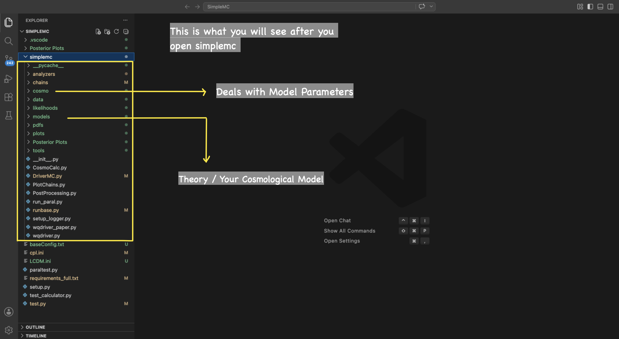
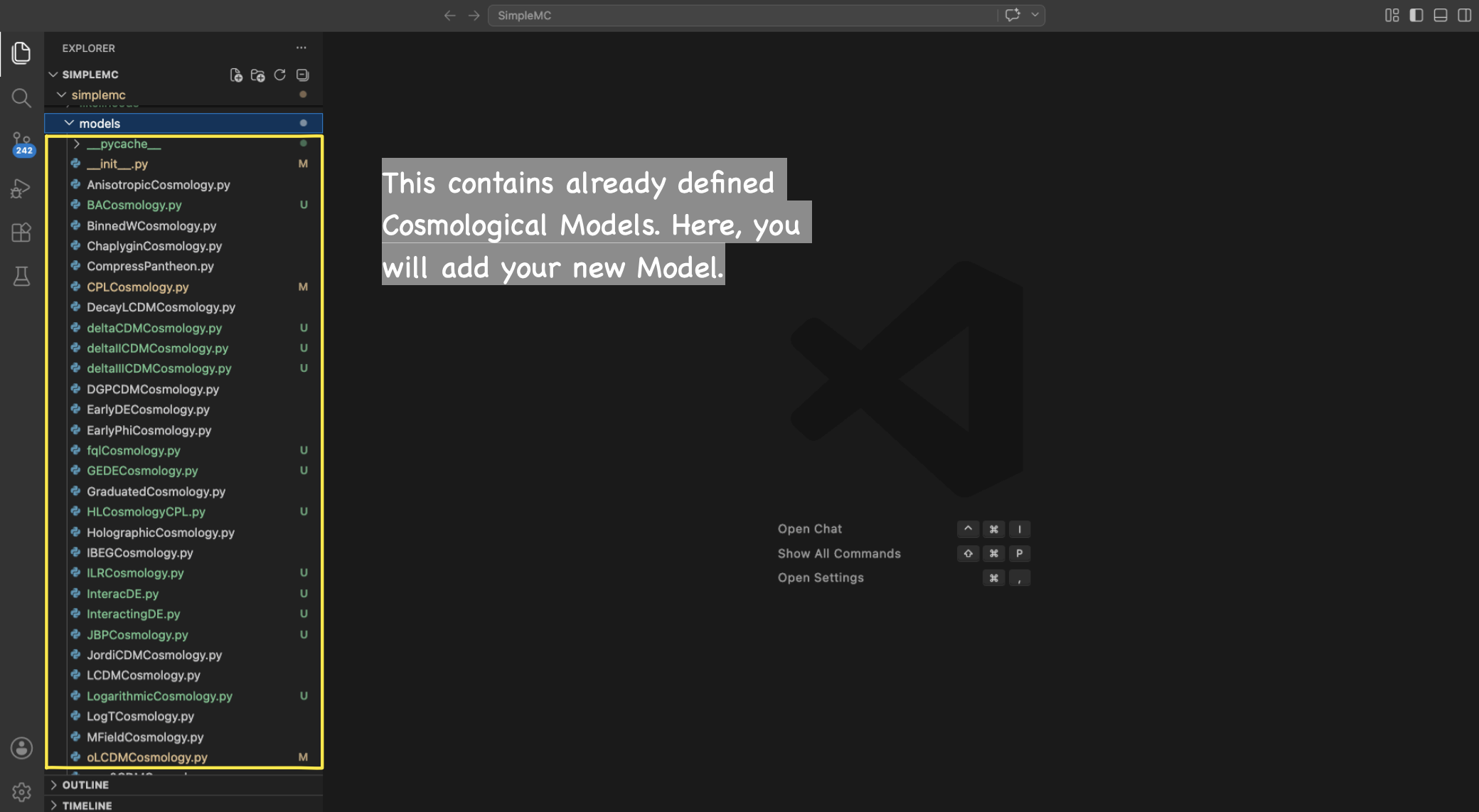
Inside the SimpleMC → simplemc → models directory, you can find the different cosmological models. This is the main location where new dark energy models and parametrizations can be added and modified.
Inside the SimpleMC → simplemc → likelihoods directory, you can find the different likelihoods. This is the main location where new likelihoods.
3. Adding a new dark energy Model in SimpleMC
Now, I will explain how we can add a new dark energy model within SimpleMC. As an example, we will consider the JBP (Jassal–Bagla–Padmanabhan) parametrization. For this, we first need to define the normalized Hubble function. In the case of the JBP model, the corresponding Hubble function is given by the following equation:
3.a Equation of State
\[w(z) = w_0 + w_a \frac{z}{(1+z)^2}\]3.b Dark Energy Density Evolution
The general dark energy density evolution is
\[f_{\rm DE}(z) = \exp\left[ 3\int_{0}^{z} \frac{1+w(z')}{1+z'}\,dz' \right].\]For the JBP parametrization, this becomes
\[f_{\rm DE}(z) = (1+z)^{3(1+w_0)} \exp\left[ \frac{3w_a z^2}{2(1+z)^2} \right]\]3.c Normalized Hubble Function
\[E^2(z) = \Omega_m(1+z)^3 + (1-\Omega_m) (1+z)^{3(1+w_0)} \exp\left[ \frac{3w_a z^2}{2(1+z)^2} \right]\]where
\[E(z)=\frac{H(z)}{H_0}.\]For the implementation in SimpleMC, we need to rewrite the normalized Hubble function in terms of the scale factor (a), where
3.d Using this relation, the normalized Hubble function can be written as
\[E^2(a) = \Omega_m a^{-3} + (1-\Omega_m) a^{-3(1+w_0)} \exp\left[ \frac{3w_a}{2}(a-1)^2 \right].\]3.e Once you have the normalized Hubble function in terms of the scale factor
First, go to the SimpleMC → simplemc → models directory and create a new .py file. For example, here I will create a file named JBPCosmology.py. In the screenshot below, you can see where this new model file should be placed.
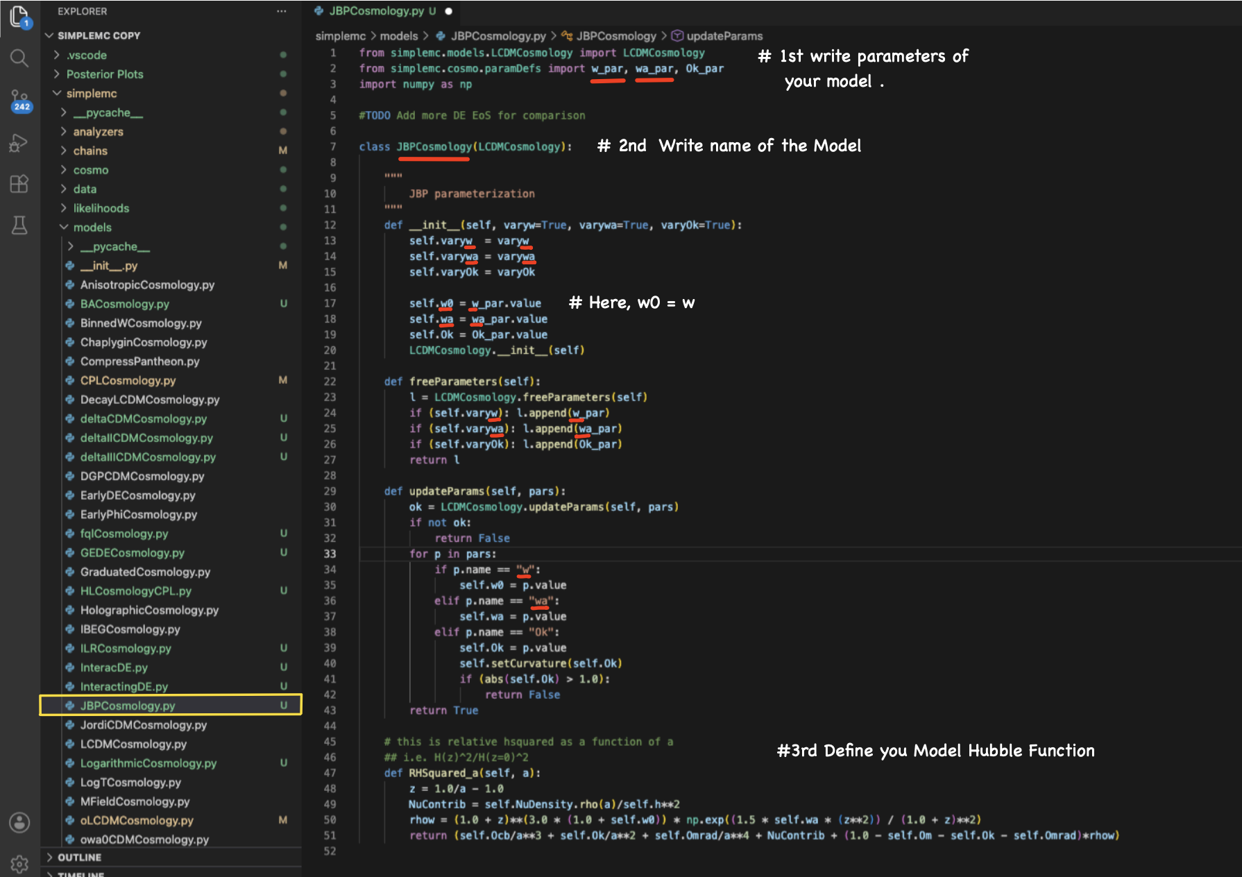
One of the most important steps is to define your model parameters. After this, you need to import the required parameters from
from simplemc.cosmo.paramDefs import (your model parameters)
Then, define your cosmological class as
class JBPCosmology(LCDMCosmology):
The class name should match the name of your .py file. For example, if your file is named JBPCosmology.py, then the class should also be named JBPCosmology.
The corresponding Python class of the JBP model can be seen below:
from simplemc.models.LCDMCosmology import LCDMCosmology
from simplemc.cosmo.paramDefs import w_par, wa_par, Ok_par
import numpy as np

#TODO Add more DE EoS for comparison

TODO Add more DE EoS for comparison

class JBPCosmology(LCDMCosmology):

    def __init__(self, varyw=True, varywa=True, varyOk=True):
        self.varyw  = varyw
        self.varywa = varywa
        self.varyOk = varyOk

        self.w0 = w_par.value
        self.wa = wa_par.value
        self.Ok = Ok_par.value
        LCDMCosmology.__init__(self)

    def freeParameters(self):
        l = LCDMCosmology.freeParameters(self)
        if (self.varyw): l.append(w_par)
        if (self.varywa): l.append(wa_par)
        if (self.varyOk): l.append(Ok_par)
        return l

    def updateParams(self, pars):
        ok = LCDMCosmology.updateParams(self, pars)
        if not ok:
            return False
        for p in pars:
            if p.name == "w":
                self.w0 = p.value
            elif p.name == "wa":
                self.wa = p.value
            elif p.name == "Ok":
                self.Ok = p.value
                self.setCurvature(self.Ok)
                if (abs(self.Ok) > 1.0):
                    return False
        return True

    # this is relative hsquared as a function of a
    ## i.e. H(z)^2/H(z=0)^2
    def RHSquared_a(self, a):
        z = 1.0/a - 1.0
        NuContrib = self.NuDensity.rho(a)/self.h**2
        rhow = (1.0 + z)**(3.0 * (1.0 + self.w0)) * np.exp((1.5 * self.wa * (z**2)) / (1.0 + z)**2)
        return (self.Ocb/a**3 + self.Ok/a**2 + self.Omrad/a**4 + NuContrib + (1.0 - self.Om - self.Ok - self.Omrad)*rhow)
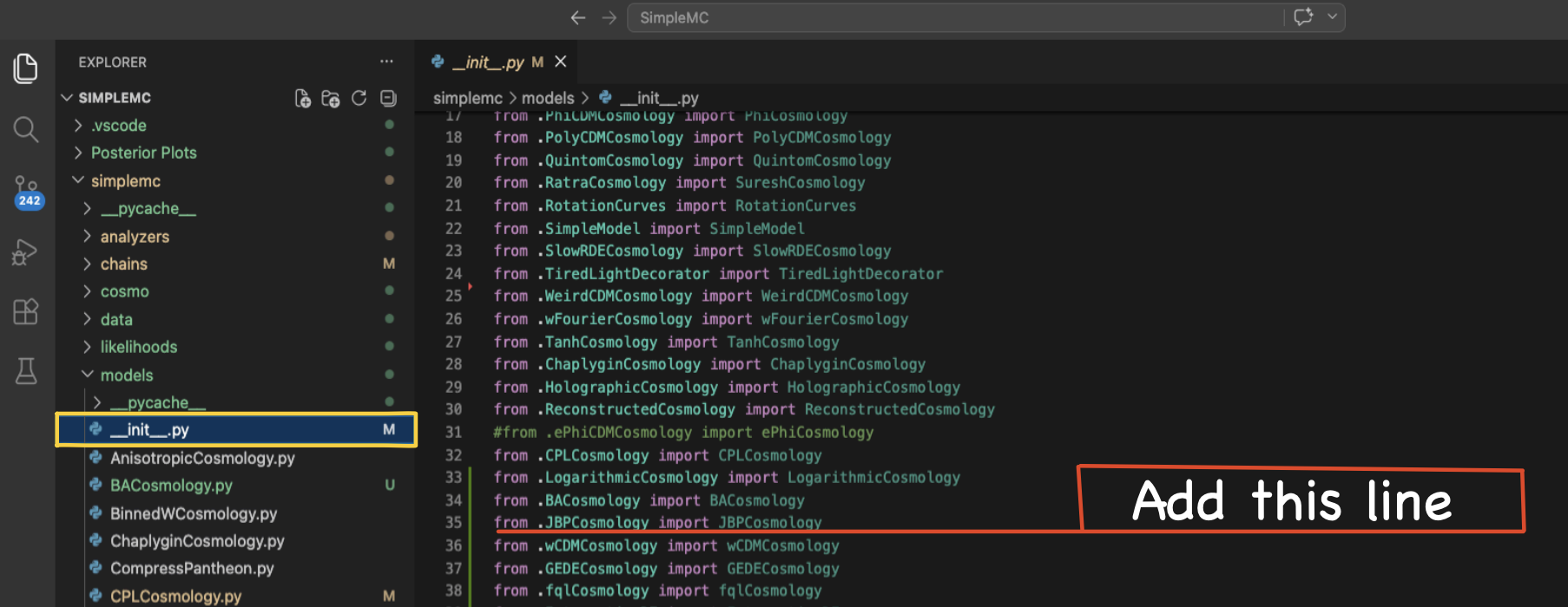
3.f Now go to the SimpleMC → simplemc → models → __init__.py
Here, you need to register your new cosmological model so that SimpleMC can recognize and import it properly.
Corresponding Python output
from .JBPCosmology import JBPCosmology
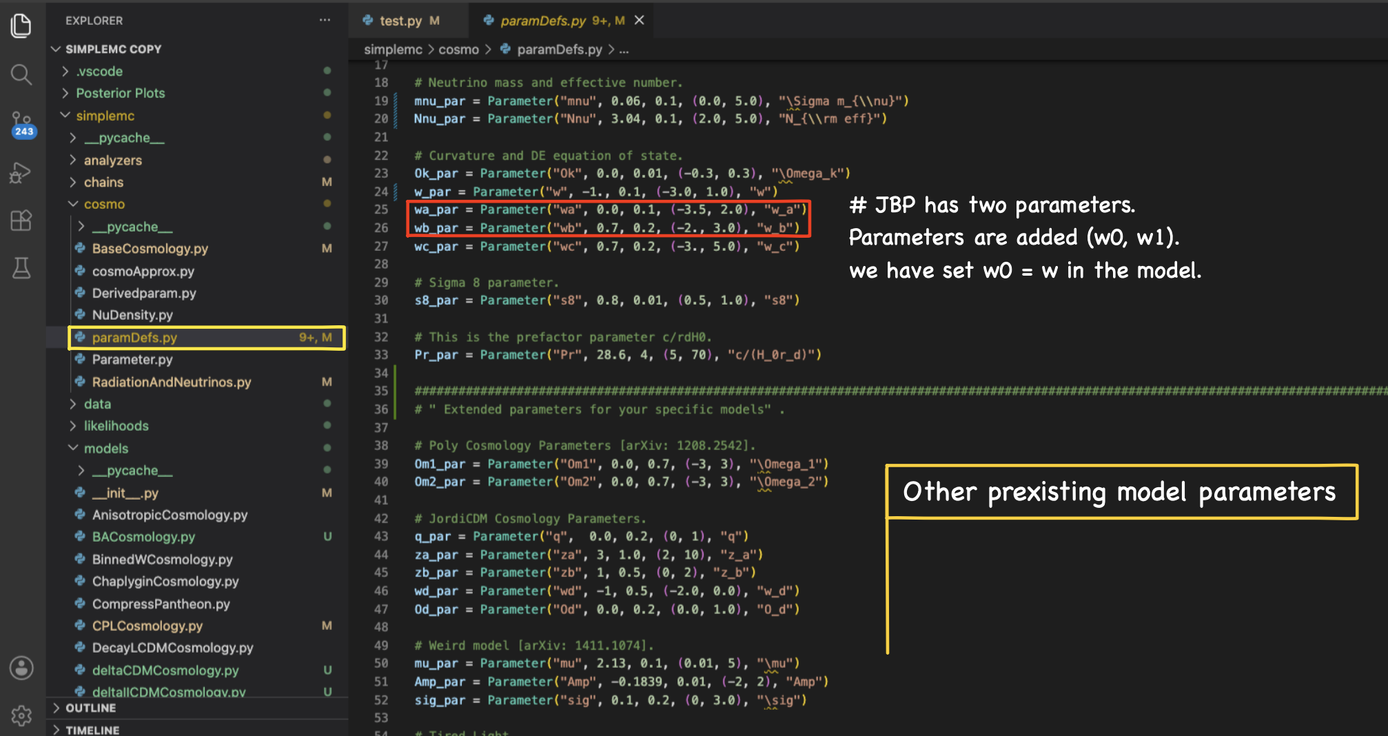
3.g Now go to the SimpleMC → simplemc → cosmo → paramDefs.py
Here, you need to define your model parameters. This means specifying the parameter name, its mean value from theory, the corresponding uncertainty, the prior range, and the LaTeX label used in plots and tables.
In general, a parameter definition looks like:
parameter_name = Parameter("parameter_name", mean_value, error, (lower_prior, upper_prior),"parameter_latex_name")
The corresponding Python parameter definitions inside paramDefs.py can be seen below:
##
# The Parameter class is defined as
# Parameter(name, value, err=0.0, bounds=None, Ltxname=None)

from simplemc.cosmo.Parameter import Parameter

# Parameters are value, variation, bounds.
# Base parameters for JBP.
Om_par = Parameter("Om", 0.3038, 0.05, (0.1, 0.5), "\Omega_m") # Matter density parameter today
Obh2_par = Parameter("Obh2", 0.02234, 0.001, (0.02, 0.025), "\Omega_{b}h^2") # Physical baryon density parameter
h_par = Parameter("h", 0.6821, 0.05, (0.4, 0.9), "h") # Dimensionless Hubble parameter
Ok_par = Parameter("Ok", 0.0, 0.01, (-0.3, 0.3), "\Omega_k") # Spatial curvature density parameter
w_par = Parameter("w", -1, 0.02, (-3.0, 1.0), "w_0") # Present value of the dark energy EoS
wa_par = Parameter("wa", 0, 0.20, (-3.0, 2.0), "w_a") # Evolution parameter of the JBP dark energy model
3.h Now go to the SimpleMC → simplemc → runbase.py
Here, we are approaching the final step before running the MCMC analysis and post-processing the results. At this stage, we need to globally register our cosmological model inside SimpleMC so that it can be directly called from the .ini configuration files and used throughout the sampling pipeline.
This can be done by adding the model inside runbase.py, as shown in the screenshot below.
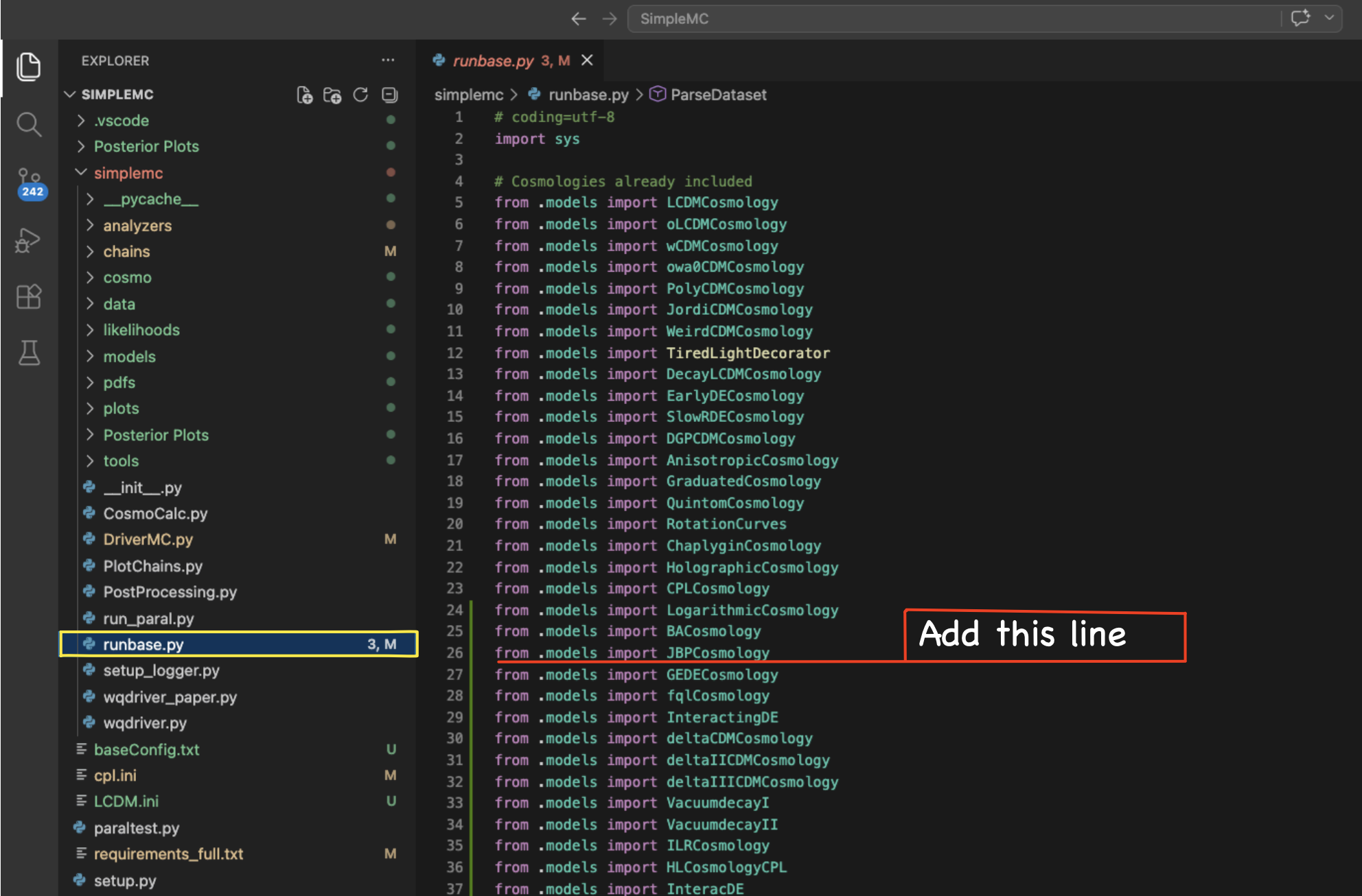
You basically need to call your model inside runbase.py using:
from .models import JBPCosmology
Now, scroll down in the same runbase.py file. Here, you need to define the global model names that will later be used inside the .ini configuration files for sampling and cosmological analyses.
Keep in mind that, while defining the JBP model, we also included the neutrino contribution through
NuContrib = self.NuDensity.rho(a)/self.h**2
Check Section 3.e, where we expressed the normalized Hubble function in terms of the scale factor (a). The same expression is implemented inside the JBPCosmology class, specifically before the definition of rhow. We also allow the curvature parameter to vary through varyOk=True. So, keep in mind that once you define your cosmological model, you will typically vary only the main cosmological parameters such as Om_par, Obh2_par, h_par, w_par, and wa_par. If you want to vary the curvature parameter, you need to call the model with the argument varyOk=True. Similarly, for varying the sum of neutrino masses, you need to use T.setVaryMnu() and for varying the effective number of relativistic species, use T.setVaryNnu() as shown in the screenshot below.
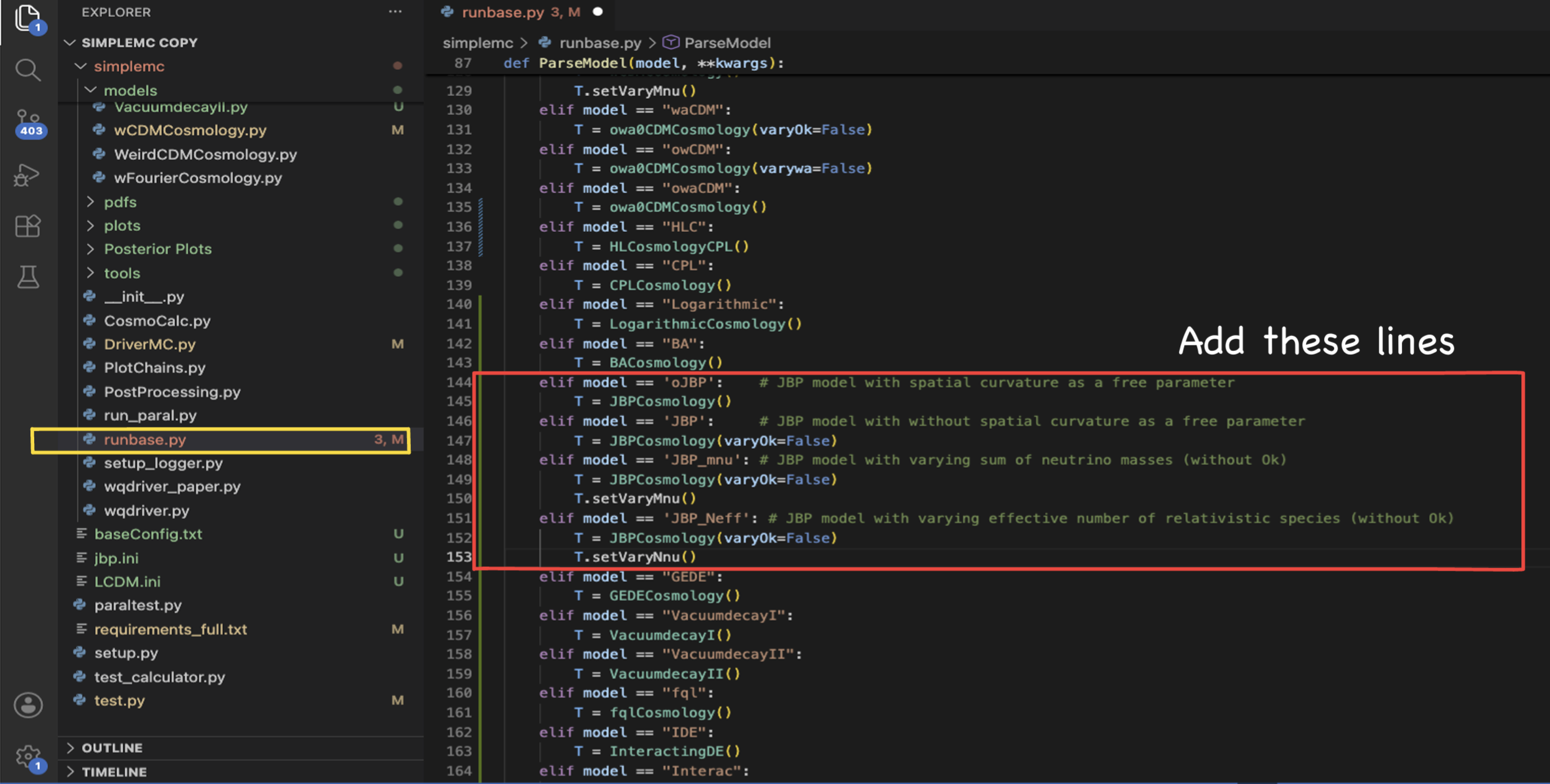
The corresponding Python implementation can be seen below:
    elif model == 'oJBP':    # JBP model with spatial curvature as a free parameter
        T = JBPCosmology()
    elif model == 'JBP':     # JBP model with without spatial curvature as a free parameter
        T = JBPCosmology(varyOk=False)
    elif model == 'JBP_mnu': # JBP model with varying sum of neutrino masses (without Ok)
        T = JBPCosmology(varyOk=False)
        T.setVaryMnu()
    elif model == 'JBP_Neff': # JBP model with varying effective number of relativistic species (without Ok)
        T = JBPCosmology(varyOk=False)
        T.setVaryNnu()
Congratulations! You have successfully defined your first cosmological model in SimpleMC. In the next page, I will show how to run the JBP model, perform post-processing of the chains, and explore the JBP parameter space using nested sampling.