Class-Installation

CLASS (Cosmic Linear Anisotropy Solving System) is a numerical tool for solving the evolution of linear cosmological perturbations and for computing the cosmological observables for a given input model. CLASS is a flexible and user-friendly code that can be easily generalized to non-minimal cosmological models. CLASS was written by Julien Lesgourgues & Thomas Tram, and first released in 2011. CLASS is written in C language for each module. It comes with C++ and Python wrapper.

For more information about CLASS can be found on the website: http://class-code.net. The CLASS papers can be found below

CLASS I: Overview, by J. Lesgourgues, arXiv:1104.2932 [astro-ph.IM]
CLASS II: Approximation schemes, by D. Blas, J. Lesgourgues, T. Tram, arXiv:1104.2933 [astro-ph.CO], JCAP 1107 (2011) 034

1. Pre-requisites

Mac users may have to install the Command Line Tools for Xcode in order to use the commands like gcc, git or make or package management tools like Homebrew. You can check if the Command Line Tools have already installed to your system or not by open the terminal and run

xcode-select -p

If they are already installed, it should return a path like /Library/Develop- er/CommandLineTools. If not, you can install them manually by running the following command

xcode-select --install

Alternatively you can download the Command Line Tools by going to the site: https://developer.apple.com/download/all/ (sign in is required), click download Command Line Tools for XCode.

Next step, you need to install Homebrew in the system. Homebrew can be downloaded it by typing this command on the terminal

/bin/bash -c "$(curl -fsSL https://raw.githubusercontent.com/Homebrew/install/HEAD/install.sh)"

After that, you will need to install a C-language compiler such as GCC (Gnu Compiler Collection), which is commonly used as a compiler with support for C, C++, Fortran, etc. GCC can be installed by compiling.

brew install gcc

To make sure that CGG works properly, run

gcc --version

Next step, check for the python version with

python --version

Python wrapper for class may not yet be compatible with Python version ? 3.11, so we have to specify version of Python in order to set up the wrapper. In this note we will use Python v.3.11. Next step, we need to install Cython. This allows Python code to directly call the C functions in CLASS. To install Cython that associate with the Python v.3.11, use the command below.

python3.11 -m pip install Cython

Linux Users
You need to have gcc compiler Python, and Cython. To install gcc use the following commands,

  sudo apt update
  sudo apt upgrade
  sudo apt install gcc

Almost every Linux distribution comes with a version of Python included in the default system packages, Check your Python version by using the following command;

  python3 --version

  python --version

In case you want a better handling of the Python packages download and install Miniconda or Anaconda from the following links; Miniconde Anaconda Next to install Cython;

  pip install Cython

  conda install Cython

2. Downloading CLASS

Before getting CLASS, you may create a project directory using

  mkdir <dirname> && cd $_

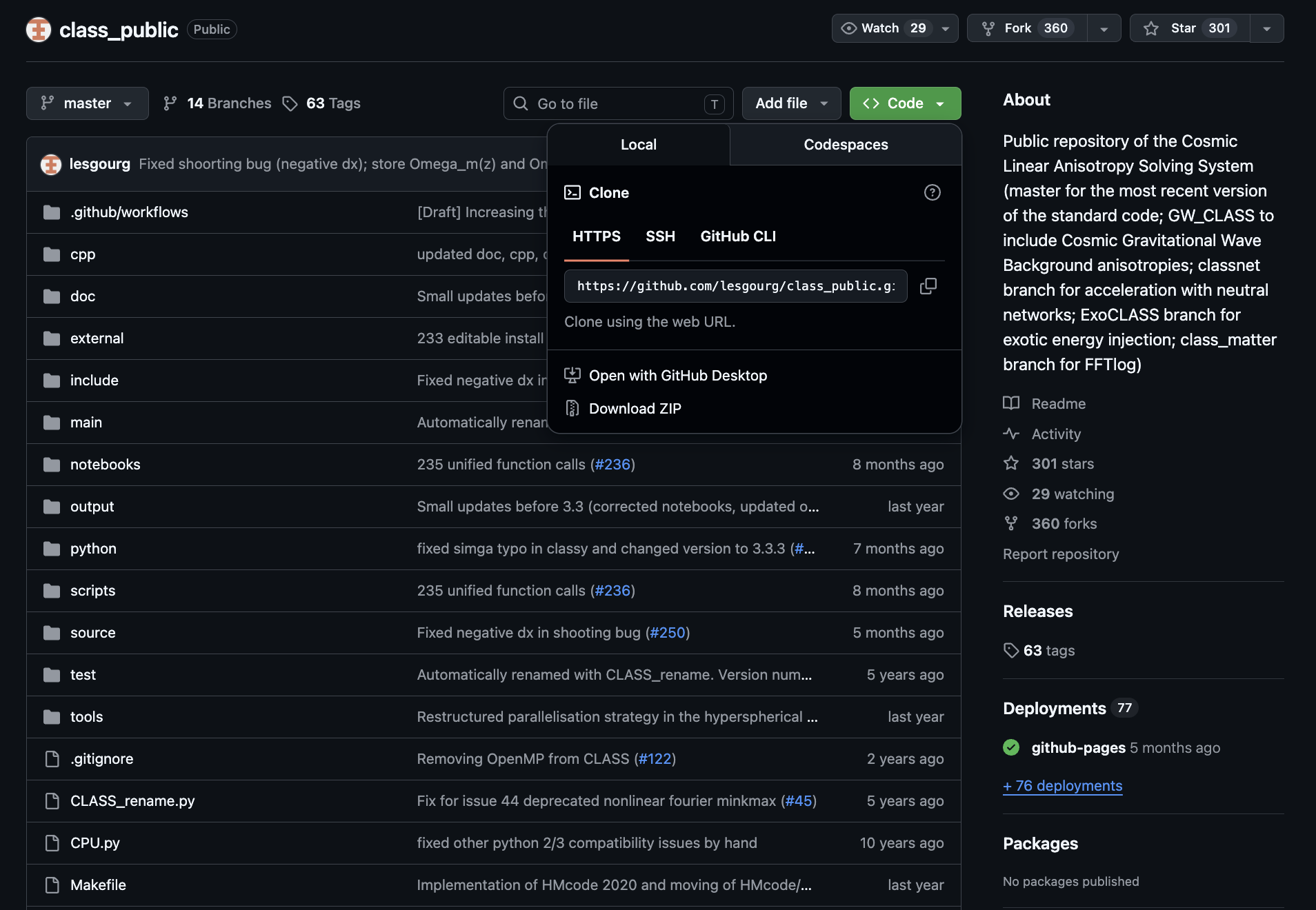
Replace with the name you prefer. After entering the directory, download the latest version of `CLASS` by downloading via git using the command

  git clone https://github.com/lesgourg/class_public.git

We can also download CLASS directly from Github.

3. Installing CLASS

Enter CLASS directory. Compile Ccode and Pythonwrapper using the command.

  PYTHON=python3.11 make all

  make -j

If you have no multiple versions of Python. Execute the command.

  ./class explanatory.ini

to test if the C code installed successfully. To test if the Python wrapper setup successfully, compile.

  python3.11 -c "import classy; print(classy.__version__)"

4. Setting Python wrapper in a virtual environment

Create a virtual environment (venv) using

  python3.11 -m venv <myenv>

You can replace <myenv> with any name you want. Then activate the virtual environment with

  source <myenv>/bin/activate

To make sure that whenever the command python is compiled it point to the correct version of Python as you included in the virtual environment, you can place the function below in .bashrc or .zshrc for z-shell (if you don’t have .bashrc or .zshrc, just create one).

  function venv() {
    source "$1/bin/activate"  
    alias python="$1/bin/python"
    alias pip="$1/bin/pip"
  }

Then restart the terminal. Activate the virtual environment again. Now you can test if the command python points to the same version of Python using in the virtual environment by compiling.

  which python; which pip

Or, check for the version of Python.

  python --version; pip --version

After that, install necessary modules to the environment, type.

  pip install numpy scipy cython matplotlib

In the CLASS directory, go to the ‘python’ directory and execute the command:

  python setup.py build
  python setup.py install

Checking if the steps above worked properly by compiling

  python -c "import classy; print(classy.__version__)"

5.Using `CLASS` on Jupyter Notebook

Firstly you have to install Jupyter Notebook.

  pip install notebook

To make sure that the path of Jupyter Notebook is in the created venv, type.

  which jupyter

If the Notebook is not in the right path, you may have follow this way:

  pip install ipython ipykernel

After installing ipython and ipykernel, run

  ipython kernel install --user --name=<myvenv>

and

  python -m ipykernel install --user --name=<myvenv>

Now the Jupyter Notebook should be in the right path. You can test it by typing (you probably have to restart the shell, and activate the venv again).

  which jupyter

If all thing going fine, to use the Jupyter Notebook, run

  jupyter notebook

(Optional) Creating the alias for the virtual environment

You can create a command to activate the venv any directory by putting the following command in the file .bashrc or .zshrc. Firstly, open the .bashrc or .zshrc file by typing

  vim ~/.bashrc

  vim ~/.zshrc

(or you can use the text editor, nano, if you prefer). Then, put the command:

  alias <your_prefer_name>="source $HOME/<path/to/myvenv>/bin/activate"

Then, overwrite the file with :wq (in vim command mode), or Ctr+O (for nano).

Monte Python

1. Getting Monte Python

MontePython can be downloaded by

  git clone https://github.com/brinckmann/montepython_public.git

You need the Python program version 2.7.x** or version 3.x**. Your Python must have ‘numpy‘ (version >= 1.4.1) and ‘Cython’. The last one is used to wrap CLASS in Python.
Optional: If you want to use the plotting capabilities of Monte Python fully, you also need the ‘scipy’, with interpolate, and ‘matplotlib’ modules.
After installation, go to the directory:

  cd montepython_public

Make a copy of the file default.conf.template and rename it to default.conf (or any name your prefer)

  cp default.conf.template default.conf

At minimum, the file default.cof needs one line.
⚠️ You need to replace <path/to/your/class_public> by your class_public installed directory path.

  path['cosmo'] = '<path/to/your/class_public>'

Make sure that your CLASS directory has the same name as in the path. Now the code is installed. There are two main (optional) commands in MontePython: the first one is run, for running MCMC to generate chains, another one is info, for analysing chains. More information can be viewed by executing

  python montepython/MontePython.py --help
  python montepython/MontePython.py run --help
  python montepython/MontePython.py info --help

To test a small running, executing:

  path['cosmo'] = '<path/to/your/class_public>'

⚠️ You need to replace <path/to/your/class_public> by your class_public installed directory path.
To get running, type:

  python montepython/MontePython.py run -o test -p input/example.param

If the directory test/ doesn’t exist, it will be created, and a run with the number of steps described in example.param will be started. To run a chain with more steps, one can type:

  python montepython/MontePython.py run -o test -p input/example.param -N 100

To analyse the chains, type

  python montepython/MontePython.py info test/

For more information, see https://baudren.github.io/montepython.html. The documentation can be found in this link.
The MontePython papers can be found as

Brinckmann, T. and Lesgourgues, J., “MontePython 3: Boosted MCMC sampler and other features”, Physics of the Dark Universe, vol. 24, 2019. doi:10.1016/j.dark.2018.100260.
Audren, B., Lesgourgues, J., Benabed, K., and Prunet, S., “Conservative constraints on early cosmology with MONTE PYTHON”, Journal of Cosmology and Astroparticle Physics, vol. 2013, no. 2, 2013. doi:10.1088/1475-7516/2013/02/001.

Setting up Planck Likelihood

The Planck 2018 data can be found on the Planck Legacy Archive. The Planck Likelihood Code (plc) is based on a library called clik. It will be extracted, alongside several clik folders that contain the likelihoods. The code uses an auto installer device, called waf.
Here is the detail of the full installation. Next, create a directory which you want to store Planck data, and go into that directory
⚠️ You need to replace <path/to/your/planck> by your own name such as planck.

  mkdir -p <path/to/planck> && cd $_

Download the code and baseline data (will need 300 Mb of space)

wget -O COM_Likelihood_Code-v3.0_R3.10.tar.gz "http://pla.esac.esa.int/pla/aio/product-action?COSMOLOGY.FILE_ID=COM_Likelihood_Code-v3.0_R3.10.tar.gz"
wget -O COM_Likelihood_Data-baseline_R3.00.tar.gz  "http://pla.esac.esa.int/pla/aio/product-action?COSMOLOGY.FILE_ID=COM_Likelihood_Data-baseline_R3.00.tar.gz"

Uncompress the code and the likelihood, and do some clean-up

  tar -xvzf COM_Likelihood_Code-v3.0_R3.10.tar.gz
  tar -xvzf COM_Likelihood_Data-baseline_R3.00.tar.gz
  rm COM_Likelihood_*tar.gz

Move into the code directory

  cd code/plc_3.0/plc-3.01

Configure the code. Note that you are strongly advised to configure clik with the Intel mkl library, and not with lapack. There is a massive gain in execution time: without it, the code is dominated by the execution of the low-l polarisation data. Before the next step, ensure you do NOT have any old Planck likelihoods sourced!

  ./waf configure --lapack_mkl=${MKLROOT} --install_all_deps

If everything goes well, you will be ready to install the code

  ./waf install

Next, source the likelihood. If you are running on a shell, type the command

  source bin/clik_profile.sh

For MacOS

Running on a z-shell, you will first need to create a .zsh version of the above file. This can be done in many ways, for example

  cp bin/clik_profile.sh bin/clik_profile.zsh
  sed -i 's/addvar PATH /PATH=$PATH:/g' bin/clik_profile.zsh
  sed -i 's/addvar PYTHONPATH /PYTHONPATH=$PYTHONPATH:/g' bin/clik_profile.zsh
  sed -i 's/addvar LD_LIBRARY_PATH/LD_LIBRARY_PATH=$LD_LIBRARY_PATH:/g' bin/clik_profile.zsh
  source bin/clik_profile.zsh

You need to add

  source </path/to/planck>/code/plc_3.0/plc-3.01/bin/clik_profile.sh

⚠️ You need to replace <path/to/your/planck> by your own installed path. to your .bashrc, and you should put it in your scripts for cluster computing.

For Ubuntu

Running on a bash-shell, you will first need to create a .sh version of the above file. This can be done in many ways, for example

  cp bin/clik_profile.sh bin/clik_profile.sh
  sed -i 's/addvar PATH /PATH=$PATH:/g' bin/clik_profile.sh
  sed -i 's/addvar PYTHONPATH /PYTHONPATH=$PYTHONPATH:/g' bin/clik_profile.sh
  sed -i 's/addvar LD_LIBRARY_PATH/LD_LIBRARY_PATH=$LD_LIBRARY_PATH:/g' bin/clik_profile.sh
  source bin/clik_profile.sh

You need to add

  source </path/to/planck/>code/plc_3.0/plc-3.01/bin/clik_profile.sh

to your .shellrc (or the .zsh to your .zshrc on a z-shell), and you should put it in your scripts for cluster computing.
After successfully installing Planck likelihoods, in MontePython configuration file, you will need to add

  path['clik'] = '</path/to/planck/code/plc_3.0/plc-3.01>'

⚠️ You need to replace <path/to/your/planck/code/plc_3.0/plc-3.01> by your own installed path.
There are nine Planck 2018 likelihoods defined in Monte Python: ‘Planck_highl_TT’, ‘Planck_highl_TT_lite’, ‘Planck_highl_TTTEEE’, ‘Planck_highl_TTTEEE_lite’, ‘Planck_lensing’, ‘Planck_lowl_TT’, ‘Planck_lowl_EE’, ‘Planck_lowl_EEBB’, ‘Planck_lowl_BB’, as well as five sets of parameter files, bestfit files, and covmats.

Class-Installation

1. Pre-requisites

2. Downloading CLASS

3. Installing CLASS

4. Setting Python wrapper in a virtual environment

5.Using CLASS on Jupyter Notebook

(Optional) Creating the alias for the virtual environment

Monte Python

1. Getting Monte Python

Setting up Planck Likelihood

5.Using `CLASS` on Jupyter Notebook