This page is devoted to macOS users with Apple Silicon chips (M1, M2, M3, and M4). In this tutorial, we will provide a step-by-step guide for installing Cobaya and its required dependencies on Apple Silicon-based Mac systems. The instructions are intended for advanced users who wish to build a fully functional environment for cosmological parameter estimation and Bayesian inference using Cobaya.
1. Installation on macOS
Install Homebrew
/bin/bash -c "$(curl -fsSL https://raw.githubusercontent.com/Homebrew/install/HEAD/install.sh)"
Install Required Compilers and Libraries
brew install wget
brew install git
brew install nano
brew install lapack
brew install cfitsio
brew install open-mpi
macOS includes a built-in Python installation, so in many cases it is not necessary to install Python through Homebrew. However, if you encounter dependency issues or version conflicts, it is recommended to install and use the Homebrew Python distribution.
Install Homebrew Python (Optional)
brew install python
python3 -m pip install --upgrade pip
You can verify the installation using
python3 --version
pip3 --version
The required Python packages such as NumPy, SciPy, Matplotlib, GetDist, MPI4Py, and other dependencies will be installed automatically during the Cobaya installation process described in the following sections.
1.a For Apple Silicon Chips
mkdir -p ~/miniconda3
curl https://repo.anaconda.com/miniconda/Miniconda3-latest-MacOSX-arm64.sh -o ~/miniconda3/miniconda.sh
bash ~/miniconda3/miniconda.sh -b -u -p ~/miniconda3
rm ~/miniconda3/miniconda.sh
source ~/miniconda3/bin/activate
1.b For Intel Chips
mkdir -p ~/miniconda3
curl https://repo.anaconda.com/miniconda/Miniconda3-latest-MacOSX-x86_64.sh -o ~/miniconda3/miniconda.sh
bash ~/miniconda3/miniconda.sh -b -u -p ~/miniconda3
rm ~/miniconda3/miniconda.sh
source ~/miniconda3/bin/activate
Before installing Cobaya, users may choose whether to install it directly in the base Conda environment or create a dedicated environment specifically for Cobaya. Using a separate environment is generally recommended because it helps avoid dependency conflicts with other scientific software.
For example, a dedicated environment can be created using:
conda create -n cobaya_env python=3.10 -y
conda activate cobaya_env
In this tutorial, however, we will proceed with the installation in the base environment for simplicity. Users who prefer an isolated setup can simply activate their custom environment before following the remaining installation steps.
2. Cobaya Installation
We begin by installing the required dependencies and the latest version of Cobaya. First, upgrade pip, install the MPI libraries (OpenMPI and mpi4py), and then install Cobaya:
python -m pip install --upgrade pip
conda install -c conda-forge openmpi mpi4py
python -m pip install cobaya --upgrade
After the installation is complete, verify that Cobaya has been installed correctly by checking its version:
python -c "import cobaya; print(cobaya.__version__)"
If the installation is successful, the command should print the installed Cobaya version without any errors. Next, create a working directory where all Cobaya-related files, chains, and configuration files will be stored:
mkdir ~/cobaya
cd ~/cobaya
3. Installing Cosmological Theory Codes and Likelihoods
Once the working directory has been created, install the cosmological theory codes and likelihood packages used by Cobaya:
cobaya-install cosmo -p ~/cobaya
cobaya-install planck_2018_highl_plik.TTTEEE
cobaya-install bicep_keck_2018
The first command downloads and installs the required cosmological theory codes and supporting packages into the ~/cobaya directory. The remaining commands install the Planck 2018 high-$\ell$ likelihood and the BICEP/Keck 2018 likelihood.
After the installation is complete, Cobaya will automatically create directories such as
~/cobaya/code
~/cobaya/data
where the external theory codes and likelihood data are stored.
Next, create a directory to store MCMC and nested-sampling chains:
mkdir ~/cobaya/chains
For users who wish to use the Cobaya graphical interface, install the required Qt package:
python -m pip install PySide6
You can then launch the graphical interface with
cobaya-cosmo-generator
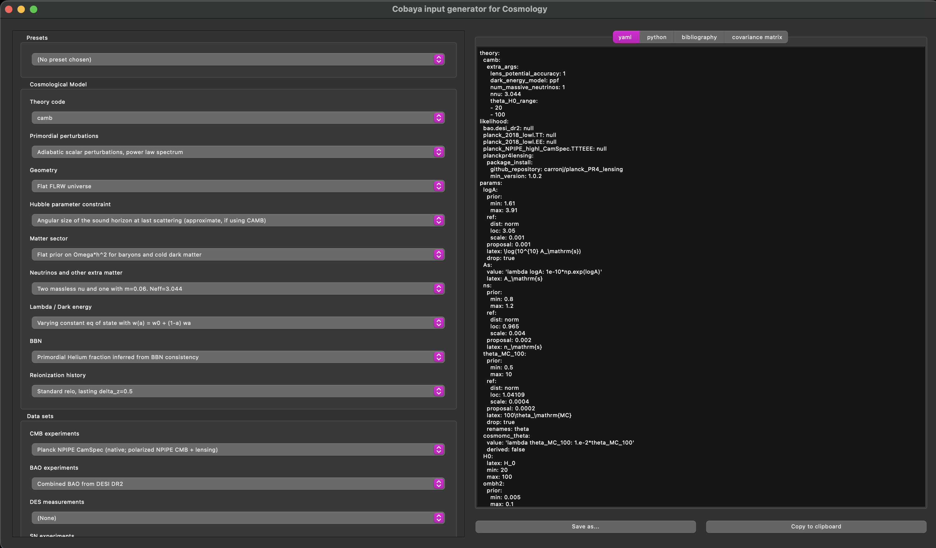
Configuration of the YAML file
theory:
  camb:
    extra_args:
      lens_potential_accuracy: 1
      dark_energy_model: ppf
      num_massive_neutrinos: 1
      nnu: 3.044
      theta_H0_range:
      - 20
      - 100
likelihood:
  bao.desi_dr2: null
  planck_2018_lowl.TT: null
  planck_2018_lowl.EE: null
  planck_NPIPE_highl_CamSpec.TTTEEE: null
  planckpr4lensing:
    package_install:
      github_repository: carronj/planck_PR4_lensing
      min_version: 1.0.2
params:
  logA:
    prior:
      min: 1.61
      max: 3.91
    ref:
      dist: norm
      loc: 3.05
      scale: 0.001
    proposal: 0.001
    latex: \log(10^{10} A_\mathrm{s})
    drop: true
  As:
    value: 'lambda logA: 1e-10*np.exp(logA)'
    latex: A_\mathrm{s}
  ns:
    prior:
      min: 0.8
      max: 1.2
    ref:
      dist: norm
      loc: 0.965
      scale: 0.004
    proposal: 0.002
    latex: n_\mathrm{s}
  theta_MC_100:
    prior:
      min: 0.5
      max: 10
    ref:
      dist: norm
      loc: 1.04109
      scale: 0.0004
    proposal: 0.0002
    latex: 100\theta_\mathrm{MC}
    drop: true
    renames: theta
  cosmomc_theta:
    value: 'lambda theta_MC_100: 1.e-2*theta_MC_100'
    derived: false
  H0:
    latex: H_0
    min: 20
    max: 100
  ombh2:
    prior:
      min: 0.005
      max: 0.1
    ref:
      dist: norm
      loc: 0.0224
      scale: 0.0001
    proposal: 0.0001
    latex: \Omega_\mathrm{b} h^2
  omch2:
    prior:
      min: 0.001
      max: 0.99
    ref:
      dist: norm
      loc: 0.12
      scale: 0.001
    proposal: 0.0005
    latex: \Omega_\mathrm{c} h^2
  omegam:
    latex: \Omega_\mathrm{m}
  omegamh2:
    derived: 'lambda omegam, H0: omegam*(H0/100)**2'
    latex: \Omega_\mathrm{m} h^2
  mnu: 0.06
  w:
    prior:
      min: -3
      max: 1
    ref:
      dist: norm
      loc: -0.99
      scale: 0.02
    proposal: 0.02
    latex: w_{0,\mathrm{DE}}
  wa:
    prior:
      min: -3
      max: 2
    ref:
      dist: norm
      loc: 0
      scale: 0.05
    proposal: 0.05
    latex: w_{a,\mathrm{DE}}
  YHe:
    latex: Y_\mathrm{P}
  Y_p:
    latex: Y_P^\mathrm{BBN}
  DHBBN:
    derived: 'lambda DH: 10**5*DH'
    latex: 10^5 \mathrm{D}/\mathrm{H}
  tau:
    prior:
      min: 0.01
      max: 0.8
    ref:
      dist: norm
      loc: 0.055
      scale: 0.006
    proposal: 0.003
    latex: \tau_\mathrm{reio}
  zrei:
    latex: z_\mathrm{re}
  sigma8:
    latex: \sigma_8
  s8h5:
    derived: 'lambda sigma8, H0: sigma8*(H0*1e-2)**(-0.5)'
    latex: \sigma_8/h^{0.5}
  s8omegamp5:
    derived: 'lambda sigma8, omegam: sigma8*omegam**0.5'
    latex: \sigma_8 \Omega_\mathrm{m}^{0.5}
  s8omegamp25:
    derived: 'lambda sigma8, omegam: sigma8*omegam**0.25'
    latex: \sigma_8 \Omega_\mathrm{m}^{0.25}
  A:
    derived: 'lambda As: 1e9*As'
    latex: 10^9 A_\mathrm{s}
  clamp:
    derived: 'lambda As, tau: 1e9*As*np.exp(-2*tau)'
    latex: 10^9 A_\mathrm{s} e^{-2\tau}
  age:
    latex: '{\rm{Age}}/\mathrm{Gyr}'
  rdrag:
    latex: r_\mathrm{drag}
sampler:
  mcmc:
    drag: true
    oversample_power: 0.4
    proposal_scale: 1.9
    covmat: auto
    Rminus1_stop: 0.01
    Rminus1_cl_stop: 0.2
After saving the .yaml file (e.g., test.yaml), run:
4. Running Cobaya
cobaya-run test.yaml
Output Files
Once the MCMC sampling with Cobaya is completed, the output consists of several files generated using the chosen run name (e.g., test). These typically include:
test.1.txt, test.checkpoint, test.covmat, test.input.yaml, test.progress, and test.updated.yaml.
Each file serves a specific purpose:
.1.txt→ Main MCMC chain file containing sampled parameter values.covmat→ Covariance matrix used for proposal updates.progress→ Information about convergence and sampling status.input.yaml/.updated.yaml→ Configuration files for the run.checkpoint→ Allows restarting the chain if interrupted
For post-processing and plotting, the most important file is:
test.1.txt
This file contains the actual MCMC samples. Inside, you will find multiple columns corresponding to different cosmological parameters (e.g., $H_0$, $\Omega_m$, $\sigma_8$, etc.), along with additional columns such as weights and likelihood values.
5. Post-processing and Visualization
Now, we introduce the main library used for post-processing, namely the GetDist package, which is widely used in cosmology. It provides a powerful and flexible framework for processing Monte Carlo chains, computing marginalized constraints, and generating high-quality plots such as one-dimensional distributions and two-dimensional contour (triangle) plots. GetDist is fully compatible with Cobaya outputs and allows efficient handling of large datasets. It also supports derived parameters, parameter transformations, and comparison between different cosmological models or datasets.
In this section, we will demonstrate how to load Cobaya chain files, analyze them using GetDist, and produce standard cosmological plots. Additional information can be found at: - GetDist Documentation, and Plot Gallery
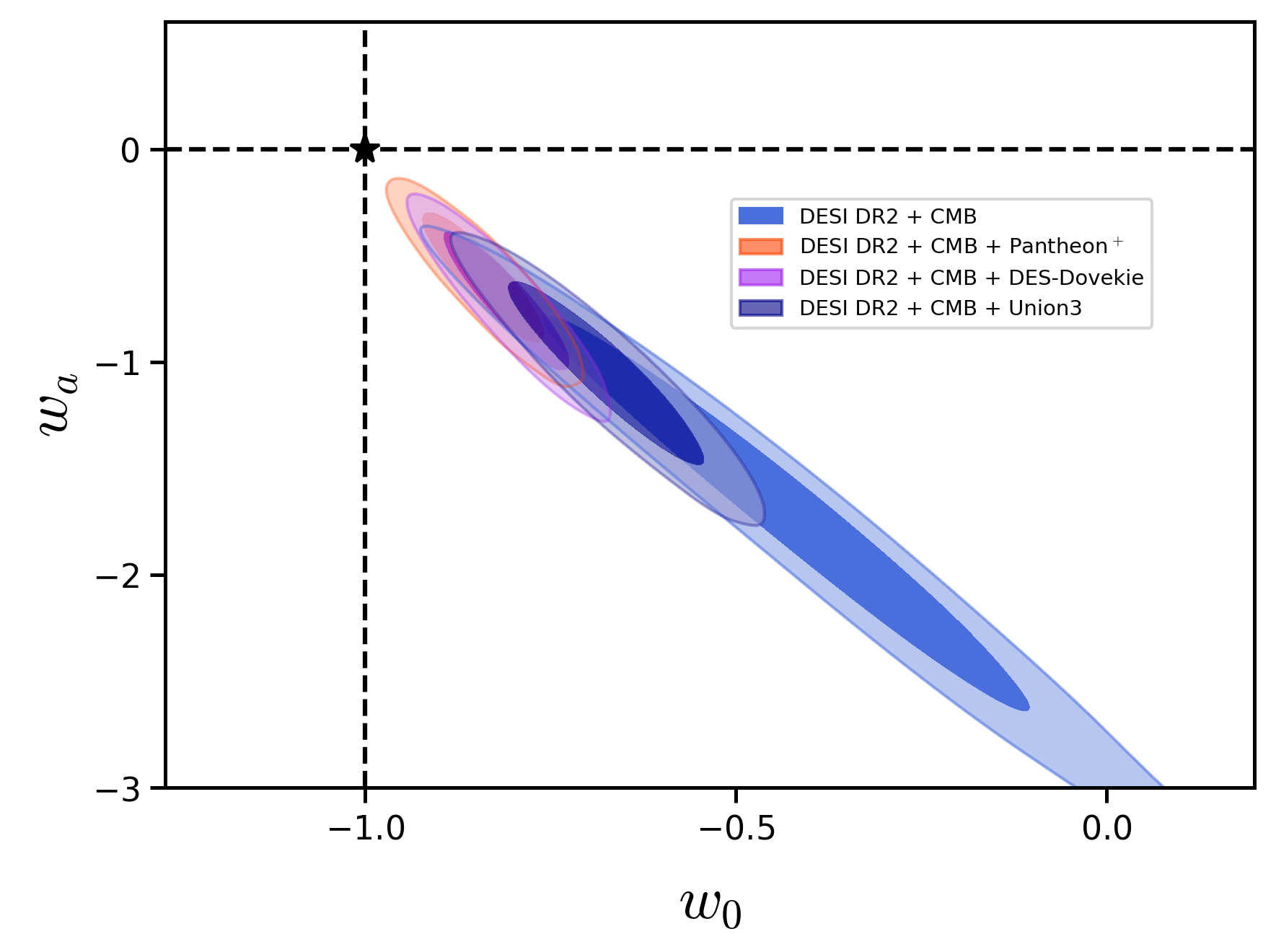
As an example, we consider the $w_0w_a$CDM model, in which the equation of state (EoS) of dark energy is parameterized as:
\[w(z) = w_0 + w_a \frac{z}{1+z}.\]Plotting with GetDist
%matplotlib inline
from getdist import plots, loadMCSamples

file_root1 = '/path/to/your/chains/test_1'
file_root2 = '/path/to/your/chains/test_2'
file_root3 = '/path/to/your/chains/test_3'
file_root4 = '/path/to/your/chains/test_4'

samples1 = loadMCSamples(file_root=file_root1, settings={'ignore_rows':0.5})
samples2 = loadMCSamples(file_root=file_root2, settings={'ignore_rows':0.5})
samples3 = loadMCSamples(file_root=file_root3, settings={'ignore_rows':0.5})
samples4 = loadMCSamples(file_root=file_root4, settings={'ignore_rows':0.5})
2D plot
g2 = plots.get_subplot_plotter(width_inch=5)
g2.settings.axes_fontsize = 16
g2.settings.axes_labelsize = 20
g2.plot_2d( [samples1, samples2, samples3, samples4], 'w0', 'wa', filled=True,
    contour_lws=1.5, colors=['#4a6fdc', '#ff4500', '#a020f0', '#00008b'])

ax = g2.subplots[0, 0]
ax.axvline(x=-1, color='black', linestyle='--', linewidth=1.5)
ax.axhline(y=0,  color='black', linestyle='--', linewidth=1.5)
ax.plot(-1, 0, marker='*', color='gold', markersize=12, zorder=10)
ax.text(-1.1, 0.1, r'$\Lambda$CDM', fontsize=12)

g2.add_legend([r'DESI DR2 + CMB',
        r'DESI DR2 + CMB + Pantheon$^+$',
        r'DESI DR2 + CMB + DES-Dovekie',
        r'DESI DR2 + CMB + Union3 '])
g2d.export("2D.png")
Triangle plot
g = plots.get_subplot_plotter(width_inch=10)
g.settings.axes_fontsize = 16
g.settings.axes_labelsize = 20
g.triangle_plot(samples1,['logA', 'ns', 'ombh2', 'omch2', 'tau', 'thetaMC', 'w0', 'wa'],legend_labels=[r'CMB + DESI DR2'],filled=True,contour_lws=1.5)
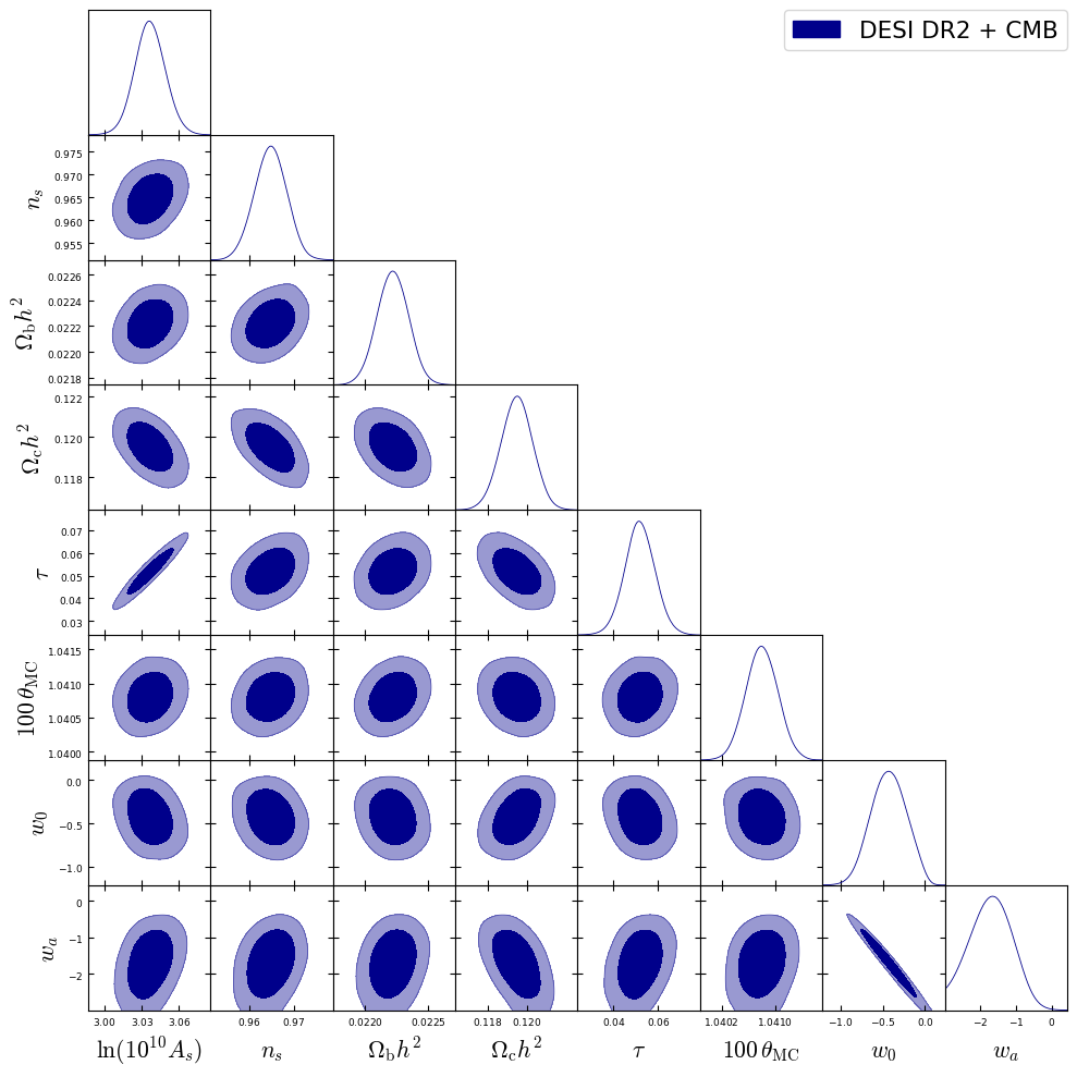
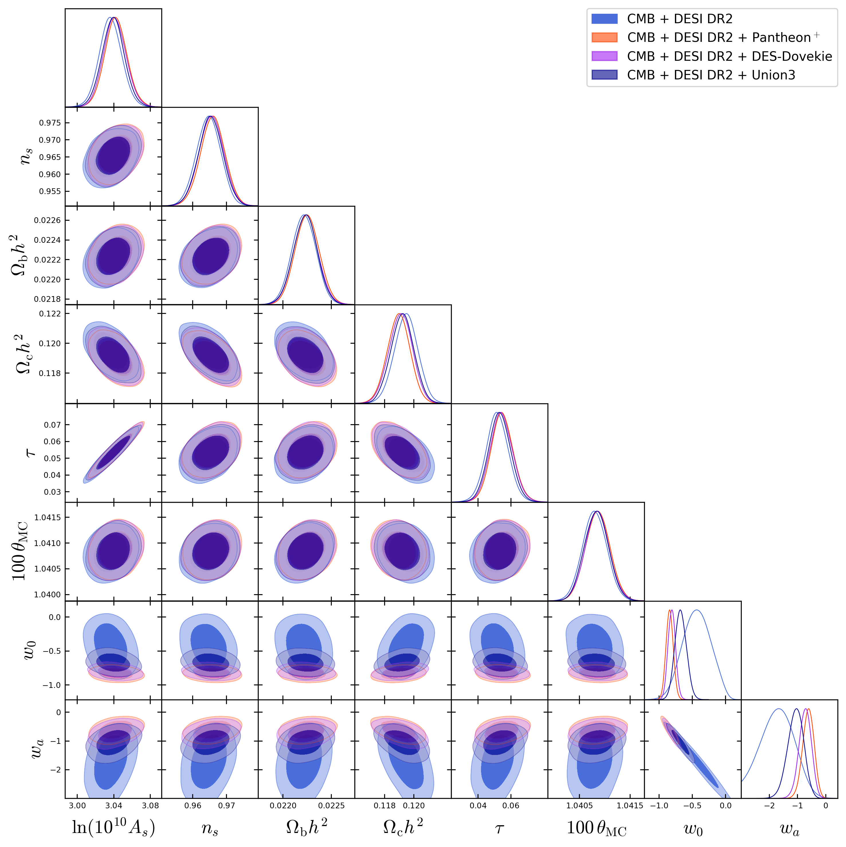
If you want to superimpose more then one chains models results, you can add additional chains to the code by including another file_root similar to the first dataset. You can also adjust the number of parameters in the same way.
%matplotlib inline
from getdist import plots, loadMCSamples

file_root1 = '/path/to/your/chains/test_1'
file_root2 = '/path/to/your/chains/test_2'
file_root3 = '/path/to/your/chains/test_3'
file_root4 = '/path/to/your/chains/test_4'

samples1 = loadMCSamples(file_root=file_root1, settings={'ignore_rows':0.5})
samples2 = loadMCSamples(file_root=file_root2, settings={'ignore_rows':0.5})
samples3 = loadMCSamples(file_root=file_root3, settings={'ignore_rows':0.5})
samples4 = loadMCSamples(file_root=file_root4, settings={'ignore_rows':0.5})

g = plots.get_subplot_plotter()

g.settings.axes_fontsize = 14
g.settings.axes_labelsize = 16
g.settings.legend_fontsize = 12
g.settings.alpha_filled_add = 0.85
g.settings.figure_legend_frame = False

g.triangle_plot(
    [samples1, samples2, samples3, samples4],
    ['logA', 'ns', 'ombh2', 'omch2', 'tau', 'thetaMC', 'w0', 'wa'],
    filled=True,
    contour_lws=1.5,
    colors=['#4a6fdc', '#ff4500', '#a020f0', '#00008b'])
g2.add_legend([r'DESI DR2 + CMB',
        r'DESI DR2 + CMB + Pantheon$^+$',
        r'DESI DR2 + CMB + DES-Dovekie',
        r'DESI DR2 + CMB + Union3 '])
g.export("fig_super.png")
The next page provides a step-by-step guide for installing Cobaya on Windows.