Implementing Different Dark Energy Models in CLASS
In the previous tutorial, we covered the installation and compilation of the CLASS and MontePython codes. With a working CLASS installation in place, we are now ready to explore one of its greatest strengths—its flexibility in implementing new dark energy models.
In this tutorial series, we will focus on modifying the CLASS source code to implement the JBP parameterization, which can be further extended to implement different dark energy models. Rather than simply replacing equations, we will first develop a clear understanding of the structure of CLASS and then, step by step, modify the CLASS code. We will also learn how cosmological parameters are passed through the code and where modifications should be introduced. This approach will make it straightforward to implement virtually any dark energy parameterization.
1. Structure of CLASS
Before modifying CLASS to implement a new dark energy model, it is important to understand how the code is organized and which files control the different stages of the cosmological calculation.
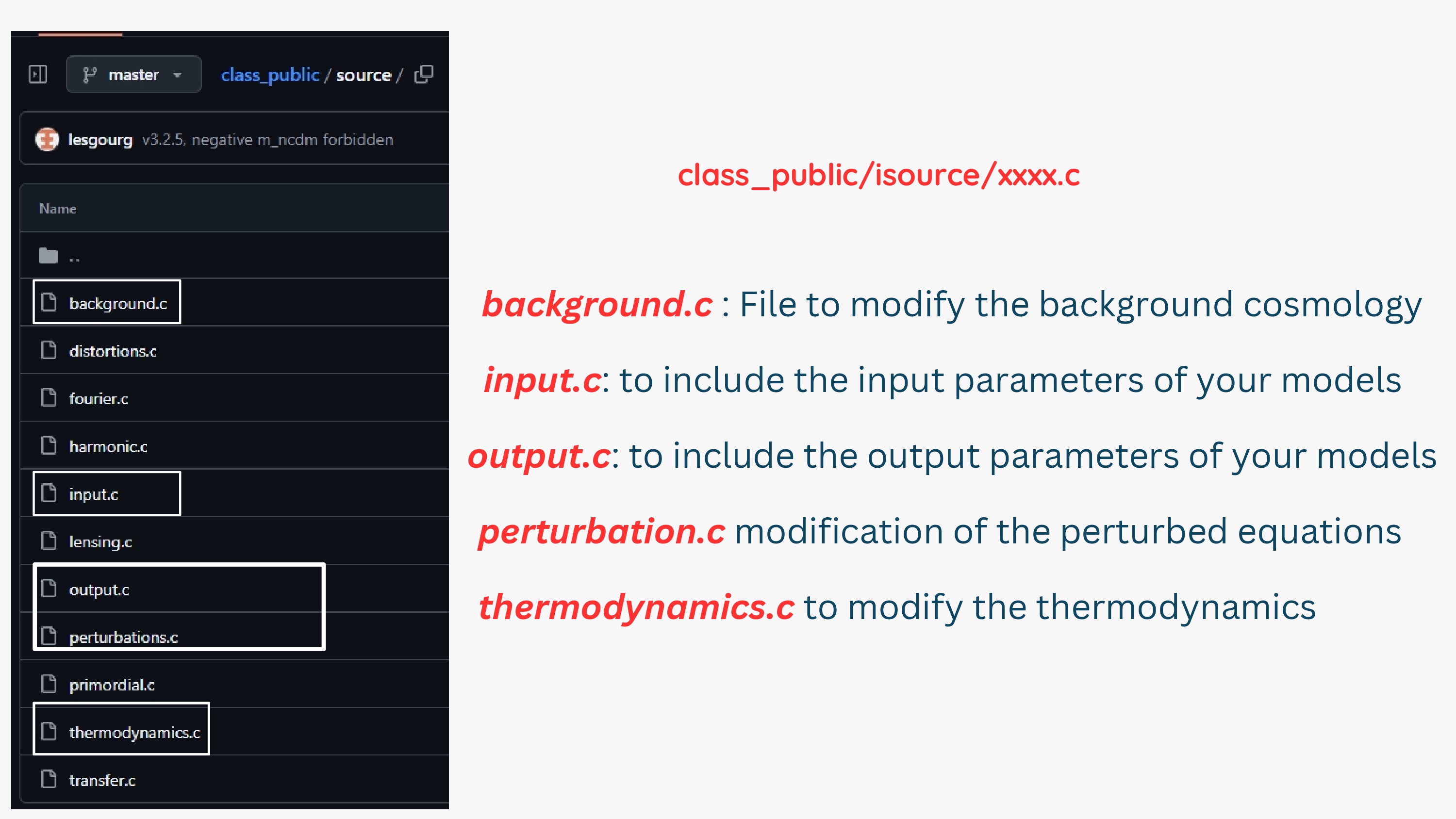
The main source files of CLASS are located in the class_public/source/ directory. CLASS follows a modular structure, where each .c file is responsible for a specific part of the calculation. For the implementation of a new dark energy model, the most relevant files are:
-
background.c— controls the background evolution of the Universe and is the main file where the background dynamics of a new dark energy model are implemented. -
input.c— reads and initializes the input parameters of the cosmological model. Any new free parameters introduced by the model must be included here. -
output.c— controls the quantities returned or written by CLASS and can be modified when new model-dependent output quantities are required. -
perturbations.c— contains the evolution equations for cosmological perturbations. This file must be considered when the new model modifies the perturbation sector. -
thermodynamics.c— handles the thermodynamic and recombination history of the Universe. Modifications are required only when the new cosmological model directly affects this sector.
The figure below highlights the main CLASS source files that may be relevant when implementing a new cosmological model.
1.1 Defining Model Parameters in background.h
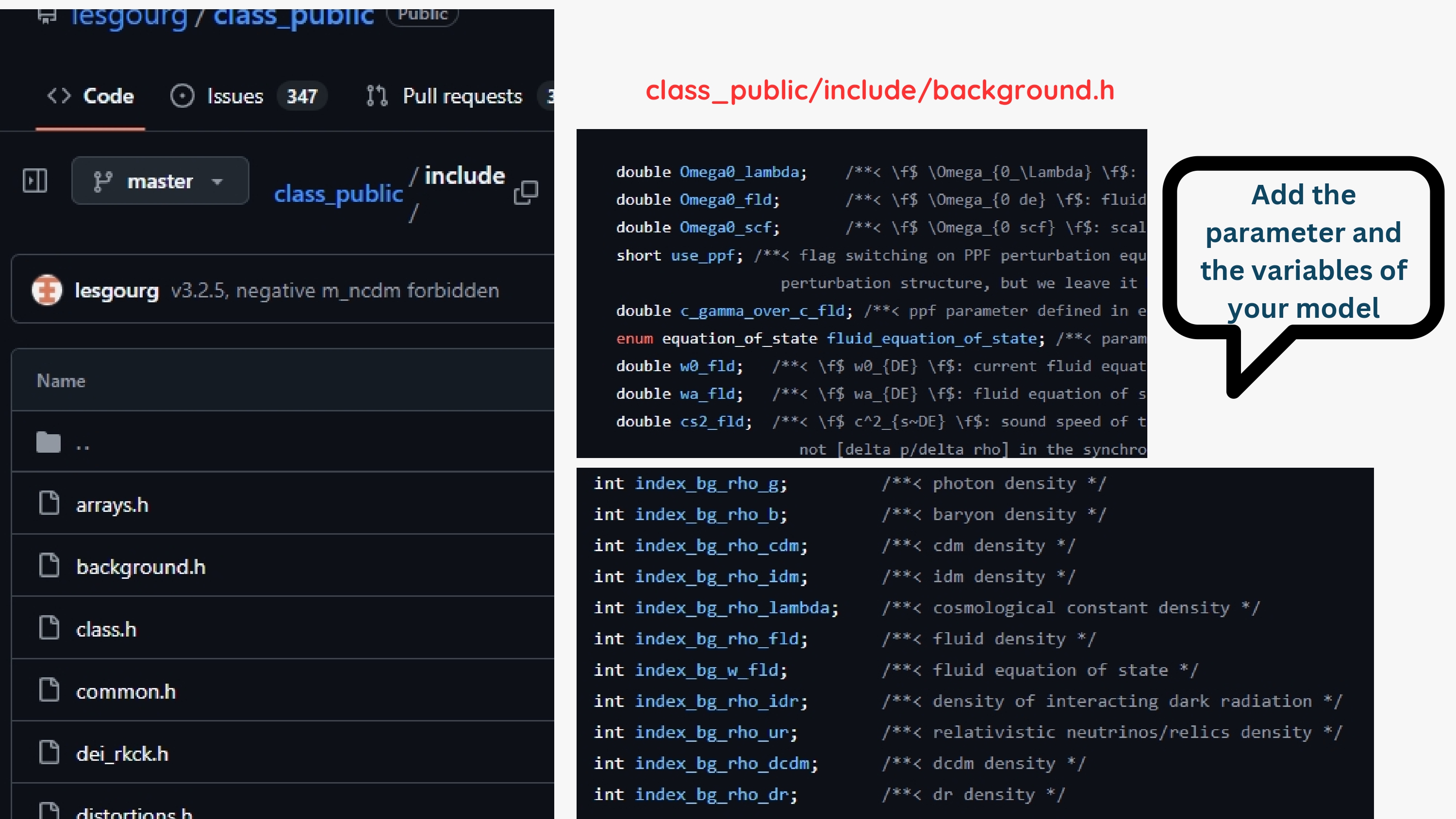
After identifying the relevant source files, the next step is to understand where the parameters and variables of a cosmological model are defined. For the background evolution, these definitions are mainly contained in
class_public/include/background.h.
The background.h header file defines the variables and indices used by the background module. For example, the standard fluid dark energy sector contains the present-day density parameter Omega0_fld, the equation-of-state parameters w0_fld and wa_fld, and the rest-frame sound speed cs2_fld.
The same file also defines indices such as index_bg_rho_fld and index_bg_w_fld, which allow CLASS to identify the corresponding quantities inside its background vectors.
Therefore, when implementing a new dark energy model that introduces additional parameters or background variables, they should first be declared in the appropriate structure in background.h. These variables can then be accessed in background.c and other CLASS modules when evaluating the cosmological evolution.
The figure below shows the relevant part of background.h, where the standard fluid dark energy parameters and background indices are defined.
1.2 Python Interface
After defining the model parameters in the CLASS header files, we also need to consider the Python interface. This interface allows the quantities defined in the C code to be accessed from Python and is essential when CLASS is used together with parameter-inference frameworks such as MontePython.
The relevant files are located in the
class_public/python/
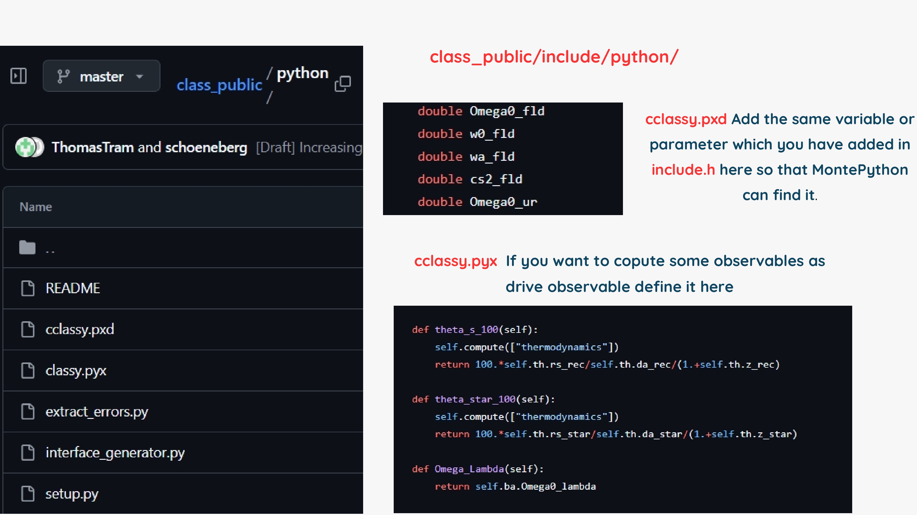
directory. Two important files for our purpose are cclassy.pxd and classy.pyx.
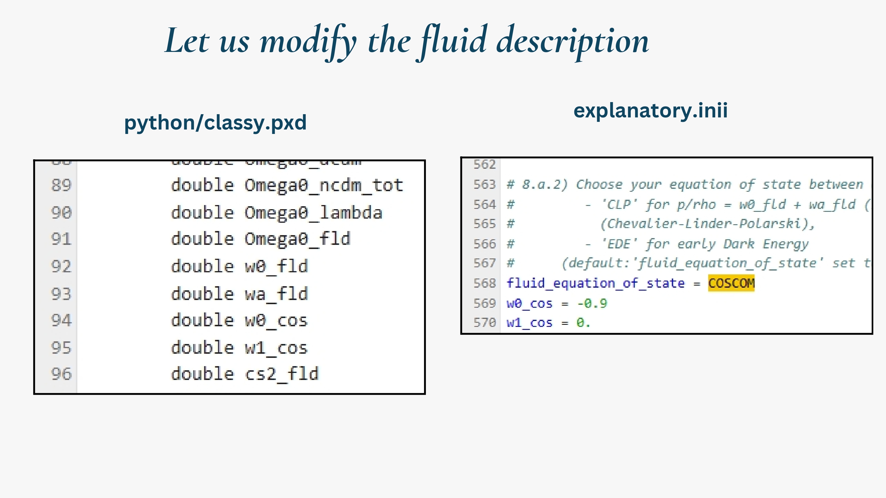
The cclassy.pxd file contains the Cython declarations of the CLASS structures. If a new model parameter has been added to a C structure, such as the background structure in background.h, the corresponding variable should also be declared in cclassy.pxd when it needs to be exposed through the Python interface. This allows the Python wrapper to recognize and access the newly introduced quantity.
The classy.pyx file defines the Python interface to CLASS. It contains functions through which different cosmological quantities can be accessed from Python. If we want to expose an additional model-dependent quantity or derived observable, an appropriate function can be defined here.
Therefore, when extending CLASS, it is important to keep the C implementation and the Python interface consistent, particularly when the modified version of CLASS will be used with MontePython.
The figure below shows the location of cclassy.pxd and classy.pyx and illustrates how CLASS variables and derived quantities can be exposed through the Python interface.
1.3 Background Evolution and Density Convention in CLASS
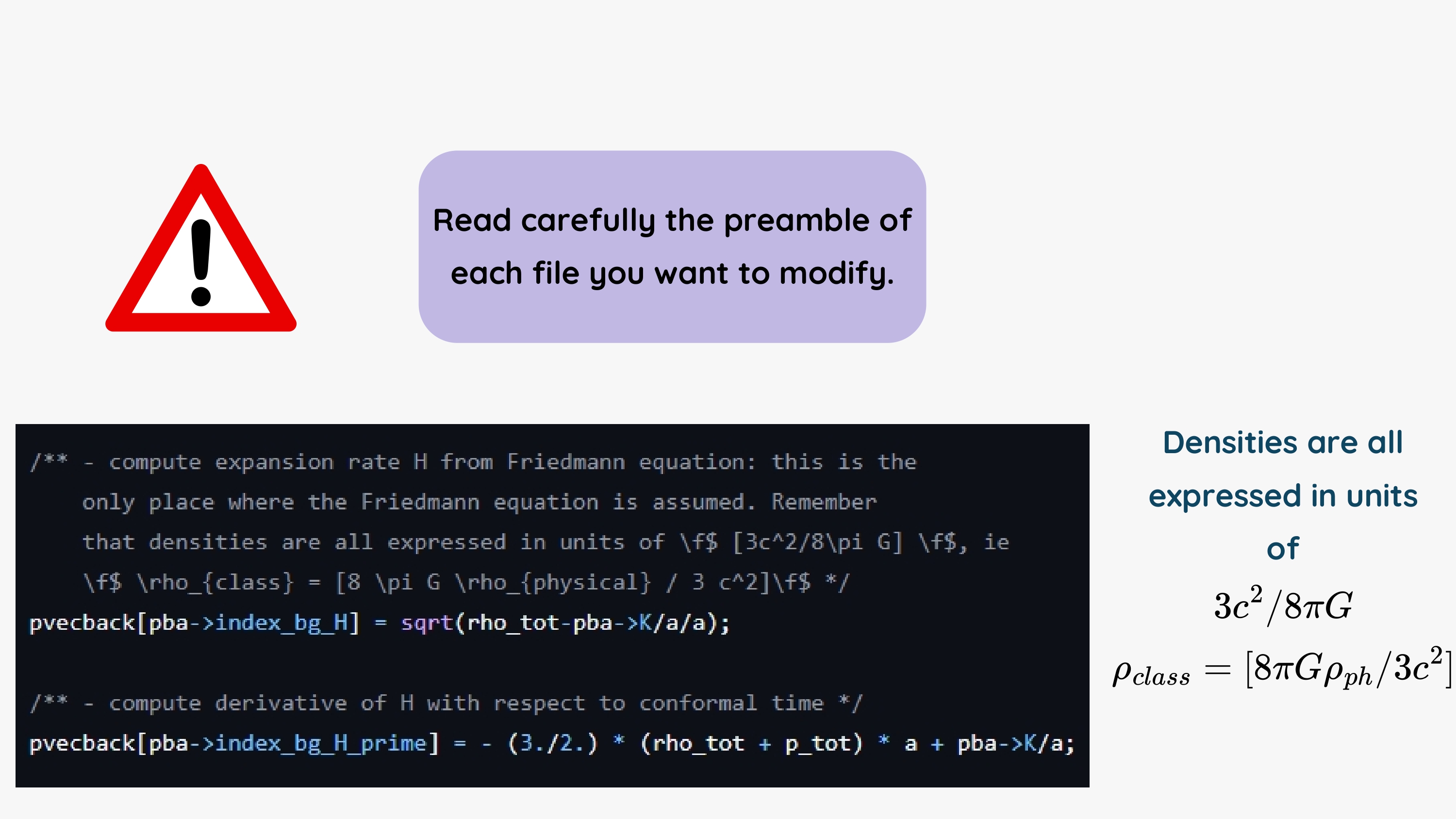
Before modifying the background equations, it is essential to understand the conventions adopted internally by CLASS. The preamble and comments provided in each CLASS source file contain important information about the definitions, units, and numerical conventions used throughout the code. Therefore, these comments should be read carefully before introducing any modification.
In background.c, the expansion rate is computed from the Friedmann equation using the total energy density of all cosmological components. CLASS internally expresses the energy densities in units of
Therefore, the physical energy density is converted according to
\[\rho_{\rm CLASS} = \frac{8\pi G}{3c^2}\rho_{\rm physical}.\]With this convention, CLASS evaluates the background expansion rate schematically as
\[H^2 = \rho_{\rm tot}-\frac{K}{a^2},\]where $\rho_{\rm tot}$ is the total density expressed in the internal CLASS units, $K$ denotes the spatial curvature, and $a$ is the scale factor.
The code also computes the derivative of the Hubble parameter with respect to conformal time using the total density and pressure. Consequently, any new dark energy component must contribute consistently to both rho_tot and p_tot.
This convention is particularly important when implementing a new dark energy model, since the model equations must be translated into the internal variables and units used by CLASS.
1.4 Computing the Total Density and Pressure
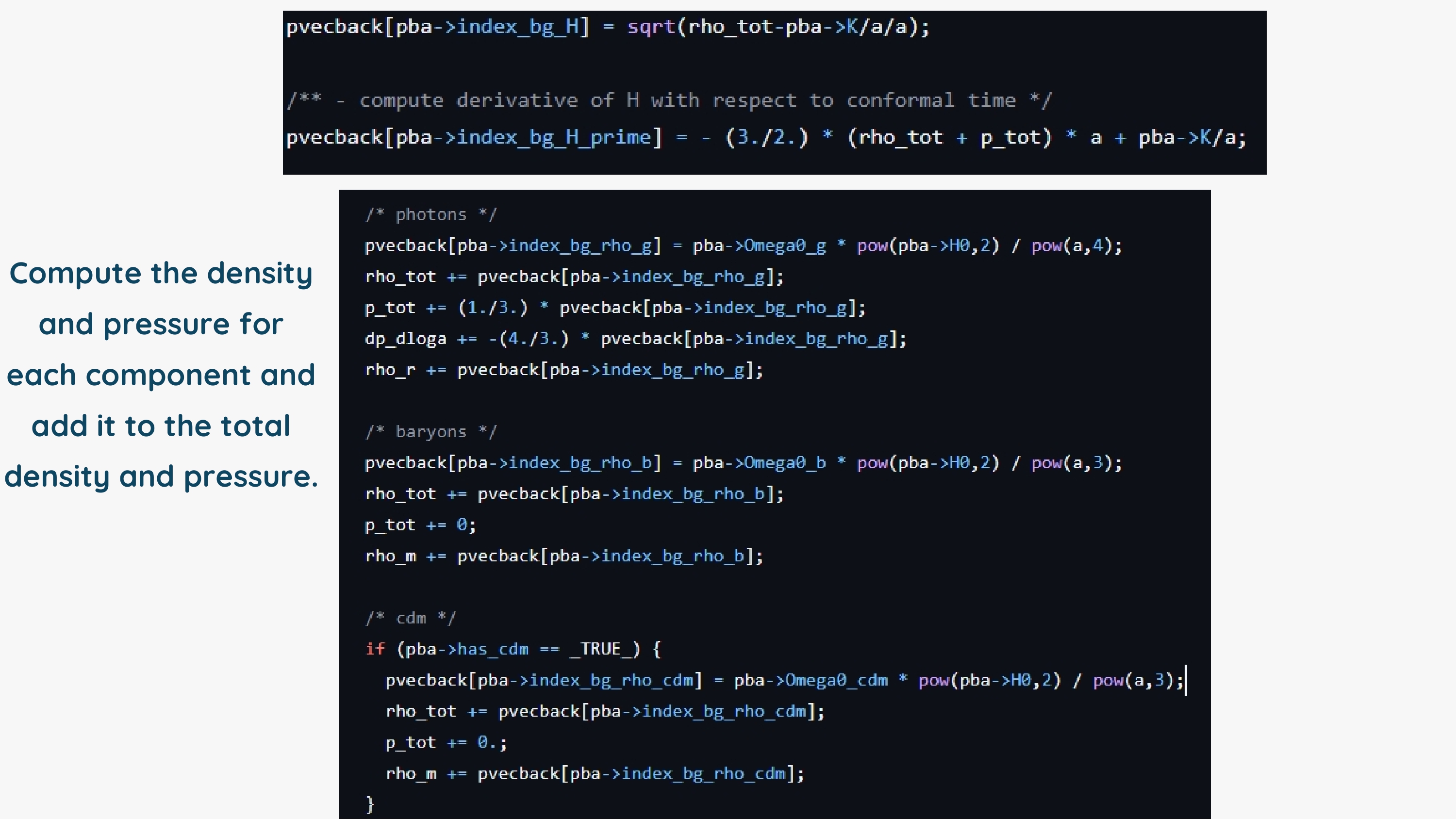
The background evolution in CLASS is constructed by computing the energy density and pressure of each cosmological component separately and then adding their contributions to the total density and pressure.
For example, the photon energy density evolves as
\[\rho_{\gamma}(a) \propto a^{-4},\]while non-relativistic components such as baryons and cold dark matter evolve as
\[\rho_{m}(a) \propto a^{-3}.\]For each component, CLASS first computes its density and stores it in the corresponding entry of the background vector pvecback. The contribution is then added to the total energy density through rho_tot. Similarly, the pressure of each component is added to p_tot.
For photons,
\[p_{\gamma} = \frac{1}{3}\rho_{\gamma},\]whereas baryons and cold dark matter are treated as pressureless components,
\[p_b = p_{\rm cdm} = 0.\]Therefore, the total background quantities are constructed schematically as
\[\rho_{\rm tot} = \rho_{\gamma} +\rho_b +\rho_{\rm cdm} +\rho_{\nu} +\rho_{\rm DE} +\cdots,\]and
\[p_{\rm tot} = p_{\gamma} +p_b +p_{\rm cdm} +p_{\nu} +p_{\rm DE} +\cdots.\]These total quantities are subsequently used by CLASS to determine the expansion history through the Friedmann equations.
This structure is particularly important for implementing a new dark energy model. Once its density $\rho_{\rm DE}(a)$ and equation of state $w_{\rm DE}(a)$ are specified, its pressure is obtained from
\[p_{\rm DE}(a) = w_{\rm DE}(a)\rho_{\rm DE}(a),\]and both contributions must be consistently included in the total background density and pressure.
The figure below illustrates how CLASS computes and accumulates the density and pressure contributions of photons, baryons, and cold dark matter.
2. Dark Energy in CLASS
Before implementing a new dark energy parameterization, it is useful to understand how dark energy is already incorporated into CLASS.
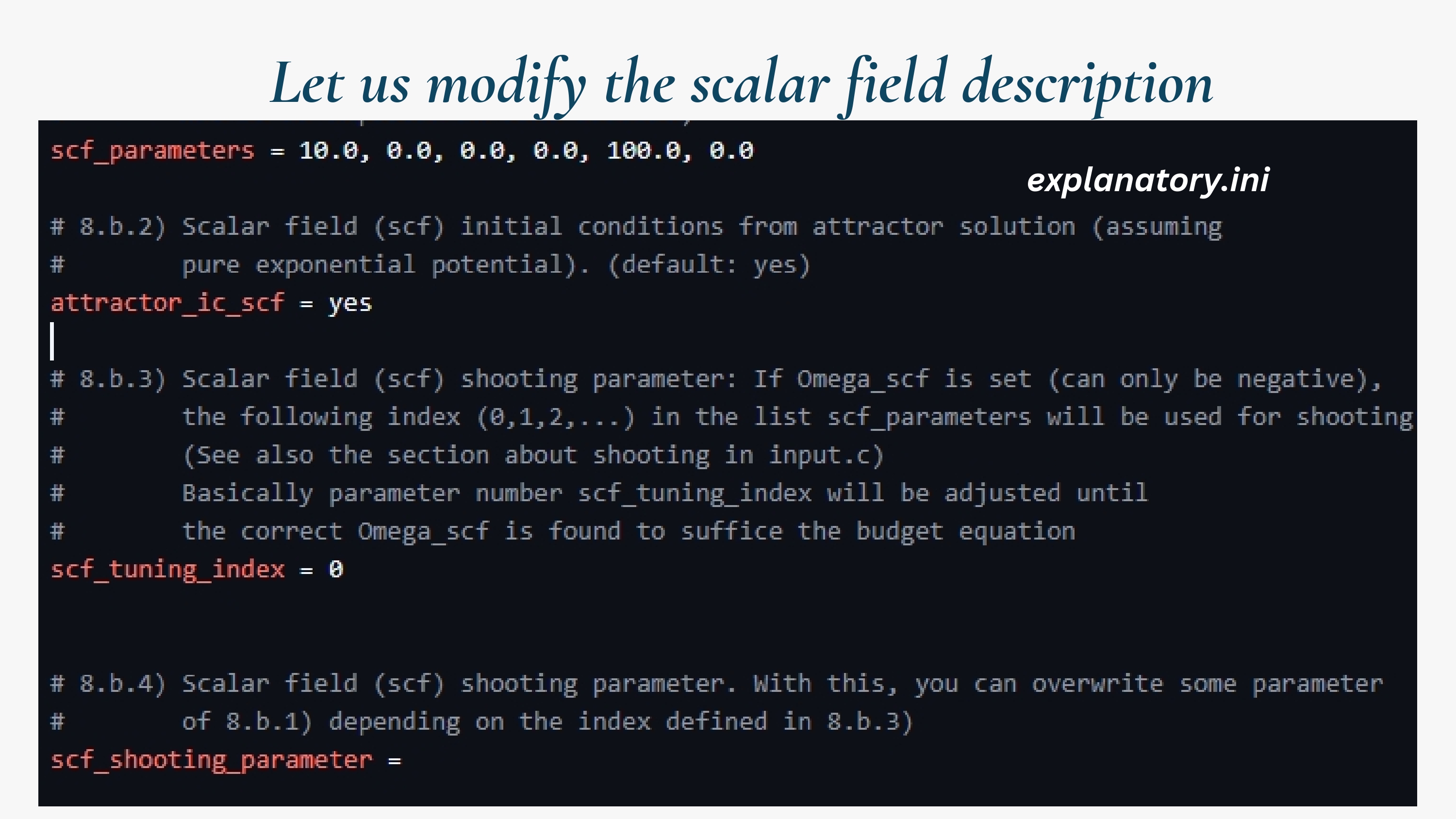
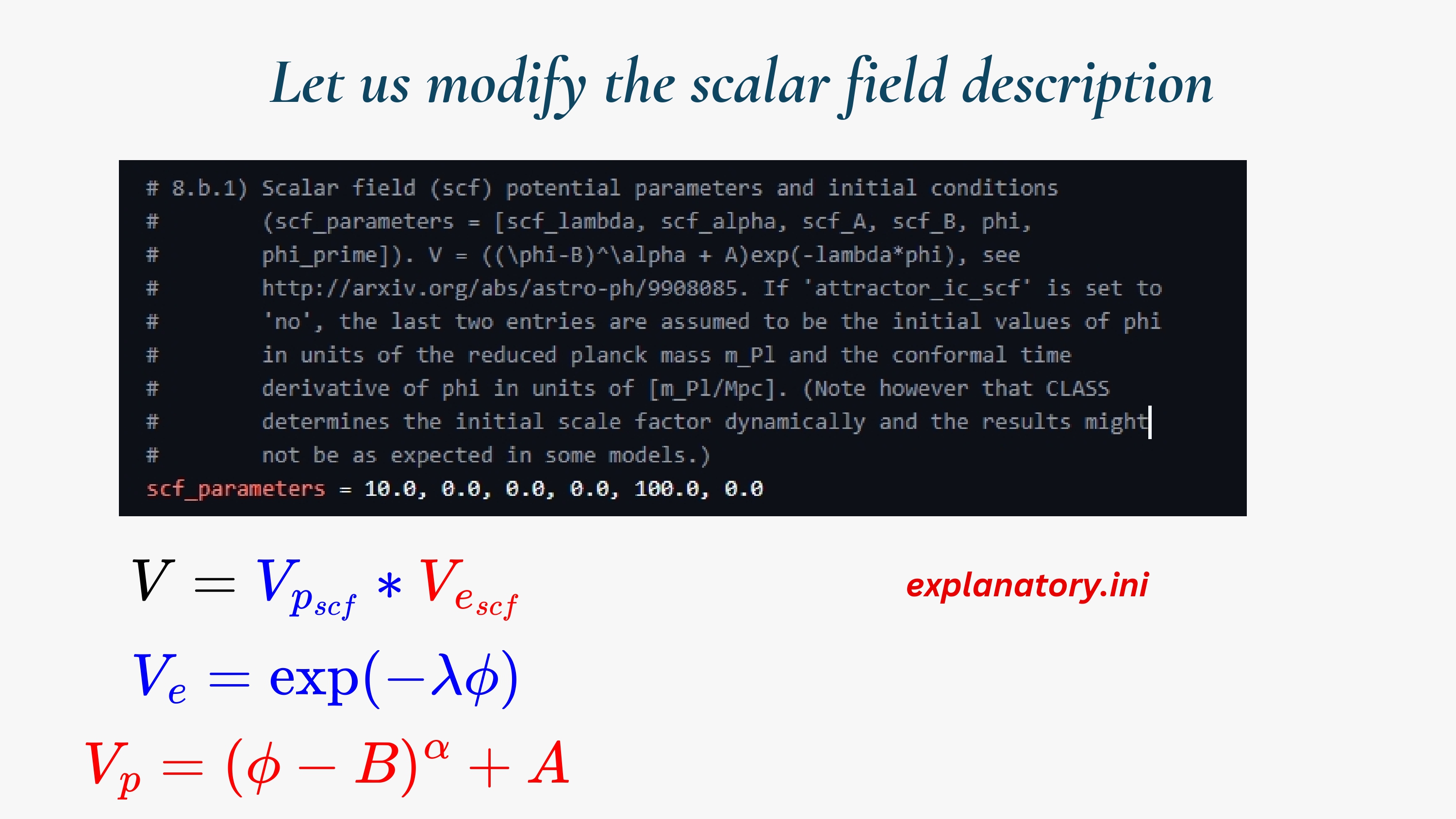
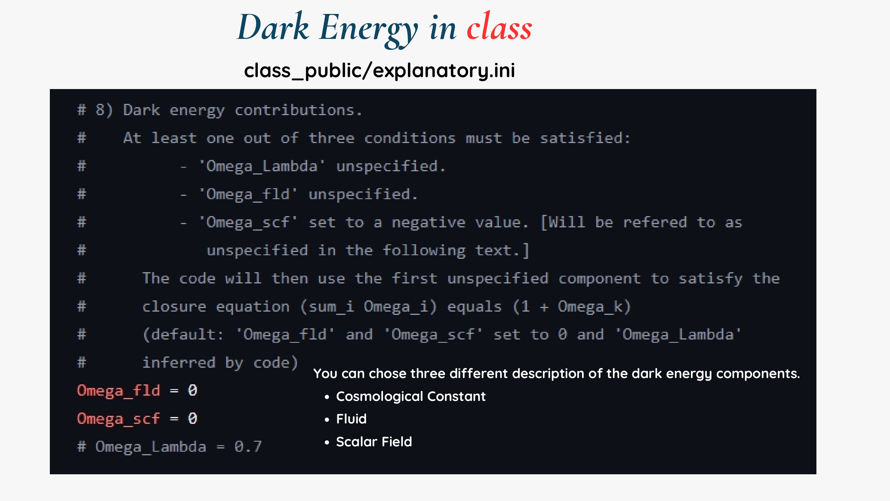
The available dark energy components and their input parameters are described in the explanatory.ini file. In the standard CLASS implementation, dark energy can be represented through three main descriptions:
- Cosmological constant (
Lambda) — corresponds to a constant vacuum-energy component with equation of state
-
Fluid (
fld) — describes dark energy as a fluid characterized by an equation of state $w(a)$. This is the sector that is particularly useful for implementing phenomenological dynamical dark energy parameterizations. -
Scalar field (
scf) — describes dark energy through the dynamics of a scalar field.
The corresponding present-day density parameters are represented internally by quantities such as Omega0_lambda, Omega0_fld, and Omega0_scf.
CLASS also uses these dark energy components when imposing the cosmological closure relation,
\[\sum_i \Omega_{i,0}=1+\Omega_{k,0},\]where $\Omega_{k,0}$ represents the present-day curvature density parameter.
If one of the dark energy density parameters is left unspecified, CLASS can infer the corresponding value from this closure condition, depending on the other components supplied in the input configuration.
For the implementation of phenomenological dark energy parameterizations such as JBP, we will mainly work with the fluid (fld) description, since it allows the dark energy equation of state to evolve with the scale factor or redshift.
The figure below shows the dark energy options described in the CLASS explanatory.ini file.
2.1 Cosmological Constant
The simplest dark energy description available in CLASS is the cosmological constant, denoted internally by Lambda. It corresponds to a constant energy density with the equation of state
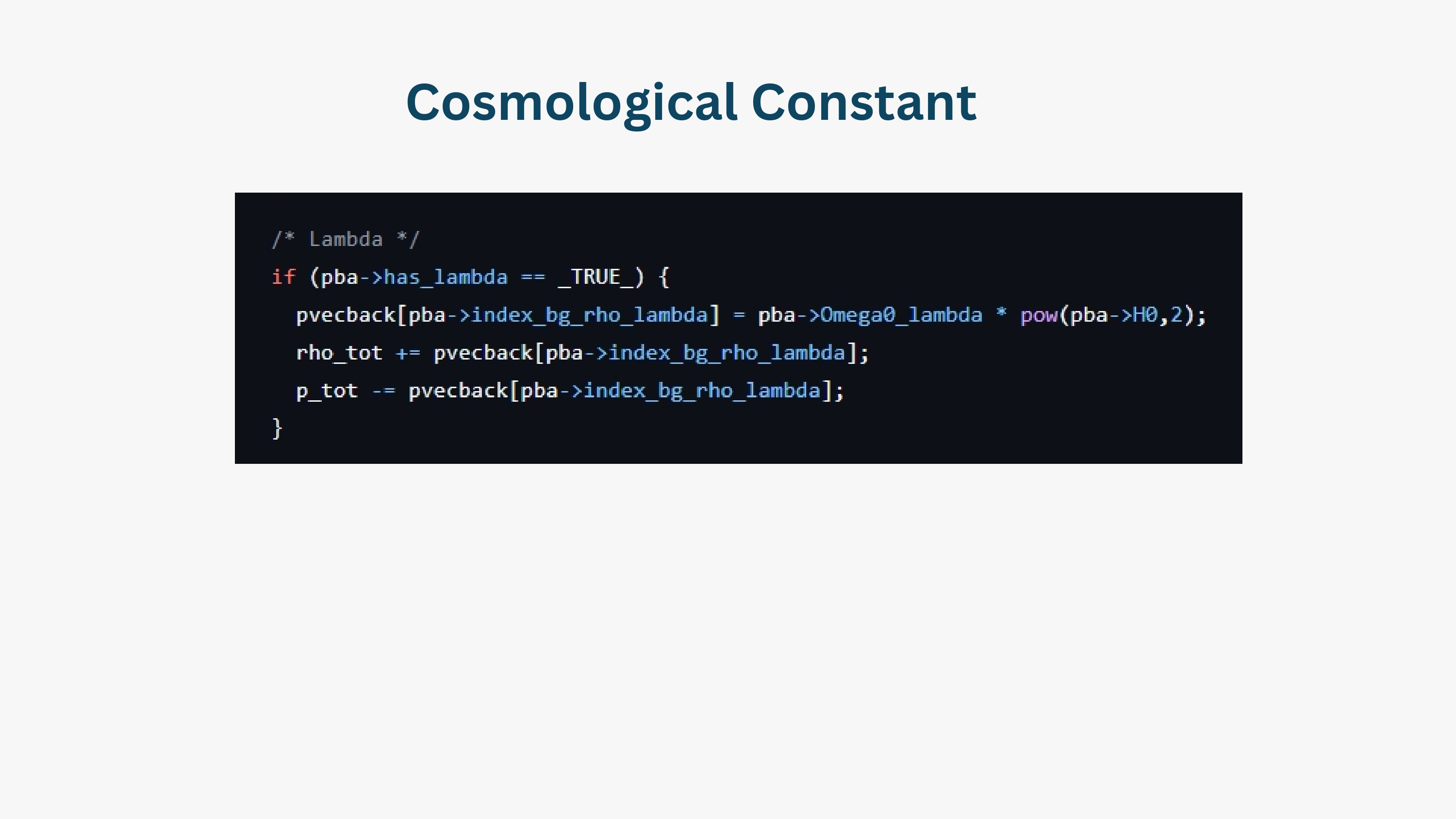
The present-day cosmological constant density is specified through Omega0_lambda. Since the energy density of a cosmological constant does not evolve with the scale factor, CLASS computes it as
in the internal CLASS density convention discussed above.
The corresponding pressure follows directly from $w_{\Lambda}=-1$,
\[p_{\Lambda}=-\rho_{\Lambda}.\]In background.c, CLASS first checks whether the cosmological constant component is active through has_lambda. Its energy density is then added to rho_tot, while the same quantity is subtracted from p_tot, thereby implementing the relation $p_{\Lambda}=-\rho_{\Lambda}$.
Thus, the cosmological constant contributes to the background evolution without introducing any time dependence in its equation of state.
The figure below shows how the cosmological constant contribution is implemented in background.c.
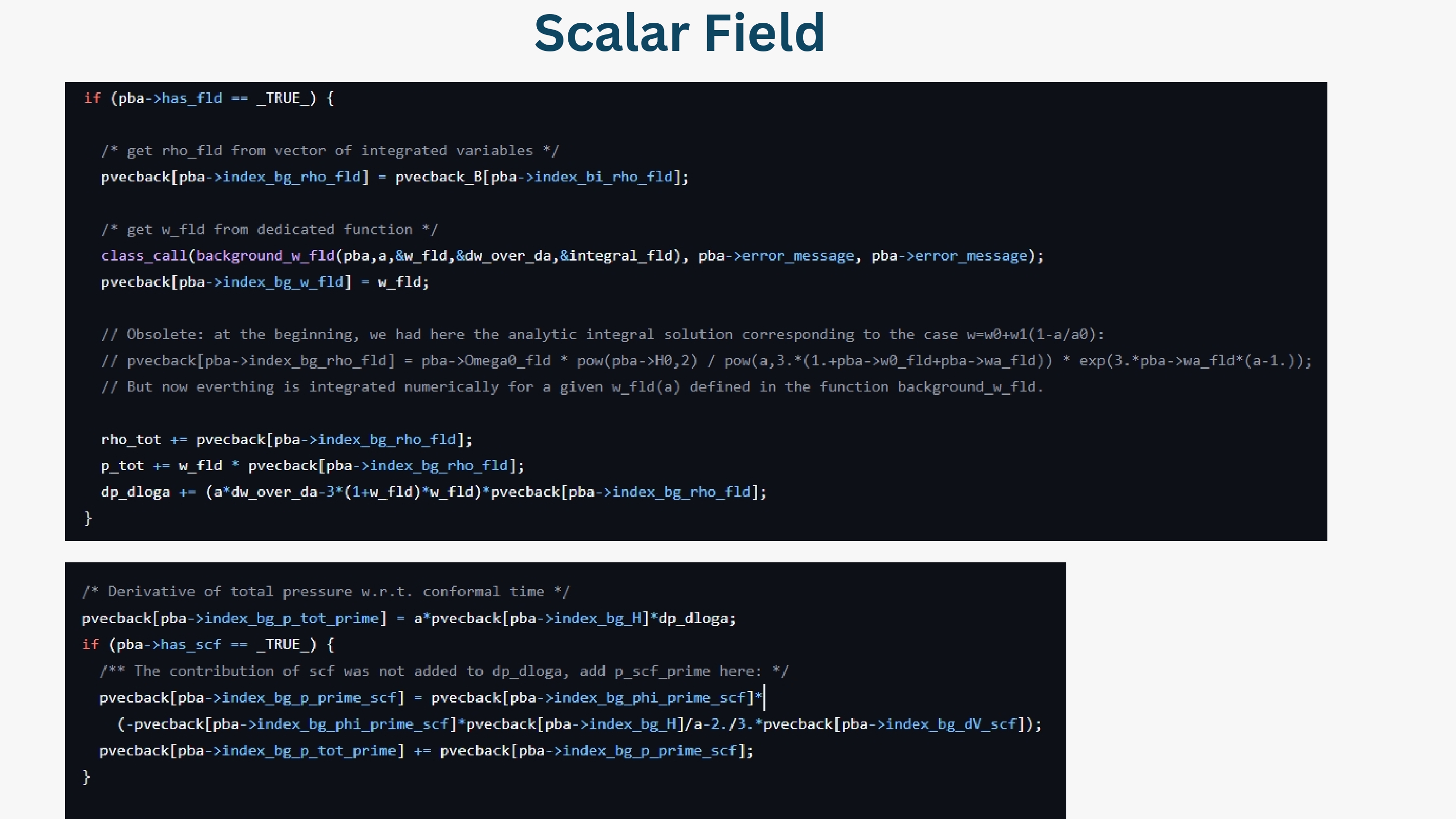
2.2 Fluid Dark Energy and Scalar-Field Contribution
In addition to the cosmological constant, CLASS allows dark energy to be described as a dynamical fluid. This sector is identified internally by fld, and it is activated when has_fld is set to _TRUE_.
Unlike the cosmological constant, the fluid component can have a time-dependent equation of state,
\[w_{\rm fld}(a) = \frac{p_{\rm fld}(a)}{\rho_{\rm fld}(a)}.\]The value of $w_{\rm fld}(a)$ is evaluated through the function background_w_fld(). This function plays a central role in implementing dynamical dark energy models because it specifies how the equation of state evolves with the scale factor.
Once $w_{\rm fld}(a)$ and $\rho_{\rm fld}(a)$ are known, CLASS adds the fluid contribution to the total energy density as
\[\rho_{\rm tot} \rightarrow \rho_{\rm tot}+\rho_{\rm fld},\]and its pressure contribution as
\[p_{\rm tot} \rightarrow p_{\rm tot} + w_{\rm fld}(a)\rho_{\rm fld}(a).\]The evolution of the fluid density follows from the continuity equation,
\[\frac{d\rho_{\rm fld}}{d\ln a} = -3\left[1+w_{\rm fld}(a)\right]\rho_{\rm fld}.\]Therefore, specifying a new function $w_{\rm fld}(a)$ determines the corresponding background evolution of the dark energy fluid.
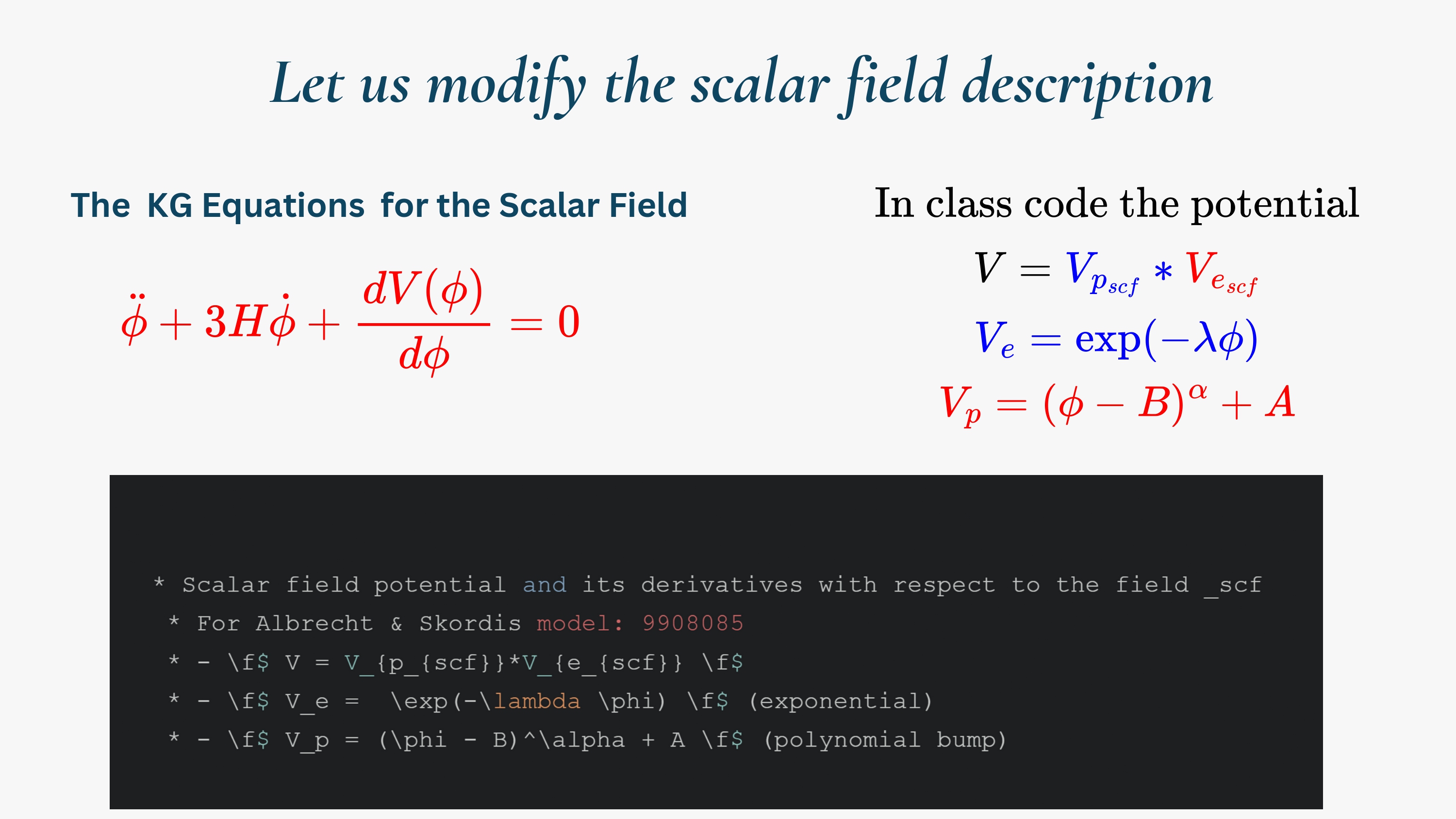
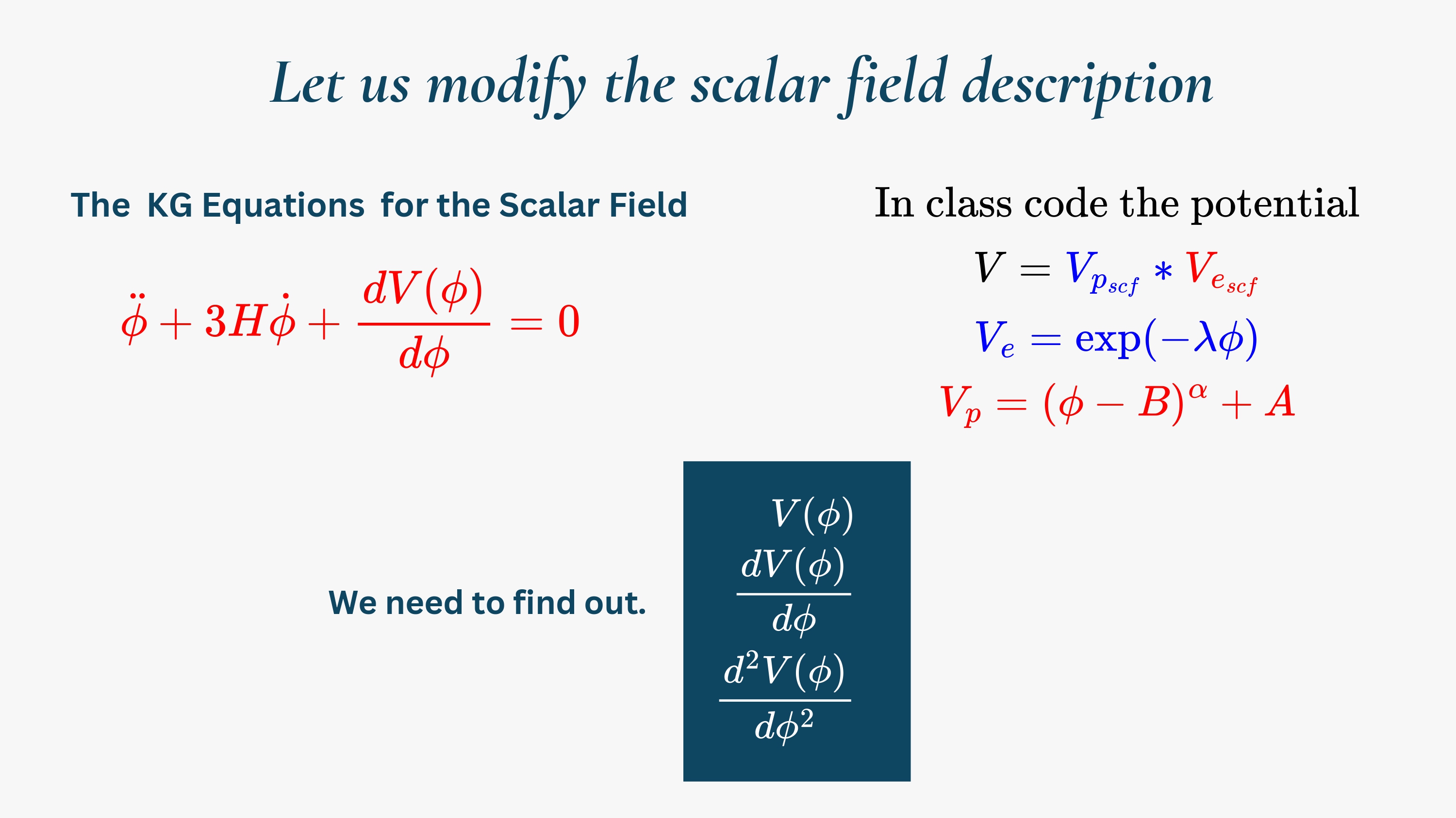
The lower part of the code also shows the treatment of the scalar-field (scf) contribution to the derivative of the total pressure. The scalar-field sector is handled separately from the phenomenological fld component.
For the JBP parameterization considered later in this tutorial, our main focus will be the fld sector, particularly the background_w_fld() function, where the desired equation of state will be introduced.
2.3 Fluid Description and the Equation of State
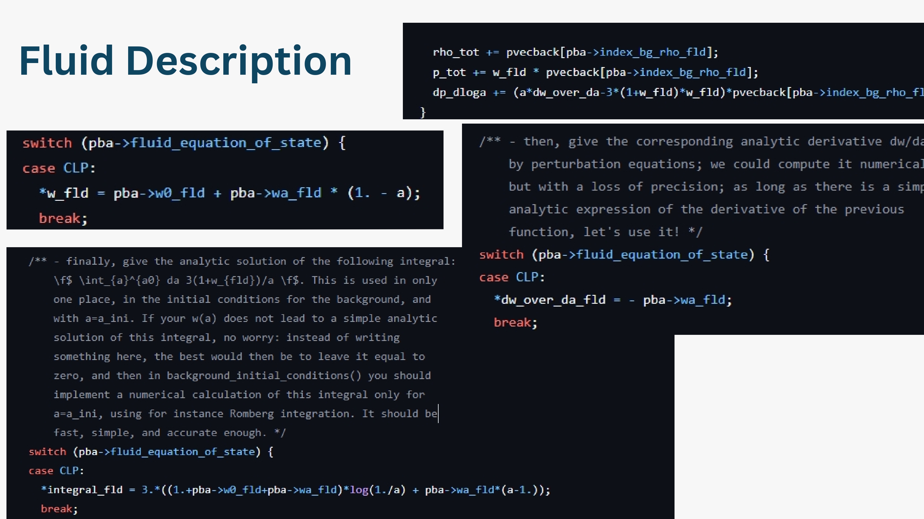
For phenomenological dynamical dark energy models, the most relevant part of CLASS is the fluid (fld) description. In this approach, the evolution of dark energy is determined by specifying its equation of state as a function of the scale factor,
In the standard CLASS implementation, one of the available fluid equations of state is the Chevallier–Polarski–Linder (CPL) parameterization,
\[w_{\rm CPL}(a) = w_0+w_a(1-a).\]This expression is implemented in the background_w_fld() function through the CLP case of fluid_equation_of_state.
In addition to $w_{\rm fld}(a)$ itself, CLASS requires its derivative with respect to the scale factor. For the CPL parameterization,
\[\frac{dw_{\rm CPL}}{da} = -w_a.\]This derivative is stored through dw_over_da_fld and is required in the evolution of the background quantities and in the perturbation equations.
The evolution of the dark energy density follows from the conservation equation,
\[\frac{d\rho_{\rm fld}}{da} = -\frac{3}{a} \left[1+w_{\rm fld}(a)\right] \rho_{\rm fld}.\]Therefore, CLASS also requires the integral
\[I(a) = \int_a^1 \frac{3\left[1+w_{\rm fld}(a')\right]}{a'} \,da'.\]For the CPL equation of state, this integral has the analytic form
\[I_{\rm CPL}(a) = 3\left[ (1+w_0+w_a)\ln\left(\frac{1}{a}\right) +w_a(a-1) \right].\]The corresponding dark energy density can then be written as
\[\rho_{\rm fld}(a) = \rho_{\rm fld,0}\, \exp\left[I(a)\right].\]Hence, when implementing a different dark energy parameterization in the fluid sector, three model-dependent quantities must be treated consistently:
- the equation of state $w_{\rm fld}(a)$,
- its derivative $dw_{\rm fld}/da$, and
- the integral $I(a)$ that determines the evolution of $\rho_{\rm fld}(a)$.
These three ingredients are the central quantities that we will modify when replacing the standard CPL parameterization with the JBP dark energy model.
2.4 Dark Energy Perturbations
So far, we have discussed how a dynamical dark energy model modifies the background evolution. However, CLASS also evolves the linear perturbations of the different cosmological components. These equations are implemented mainly in
class_public/source/perturbations.c.
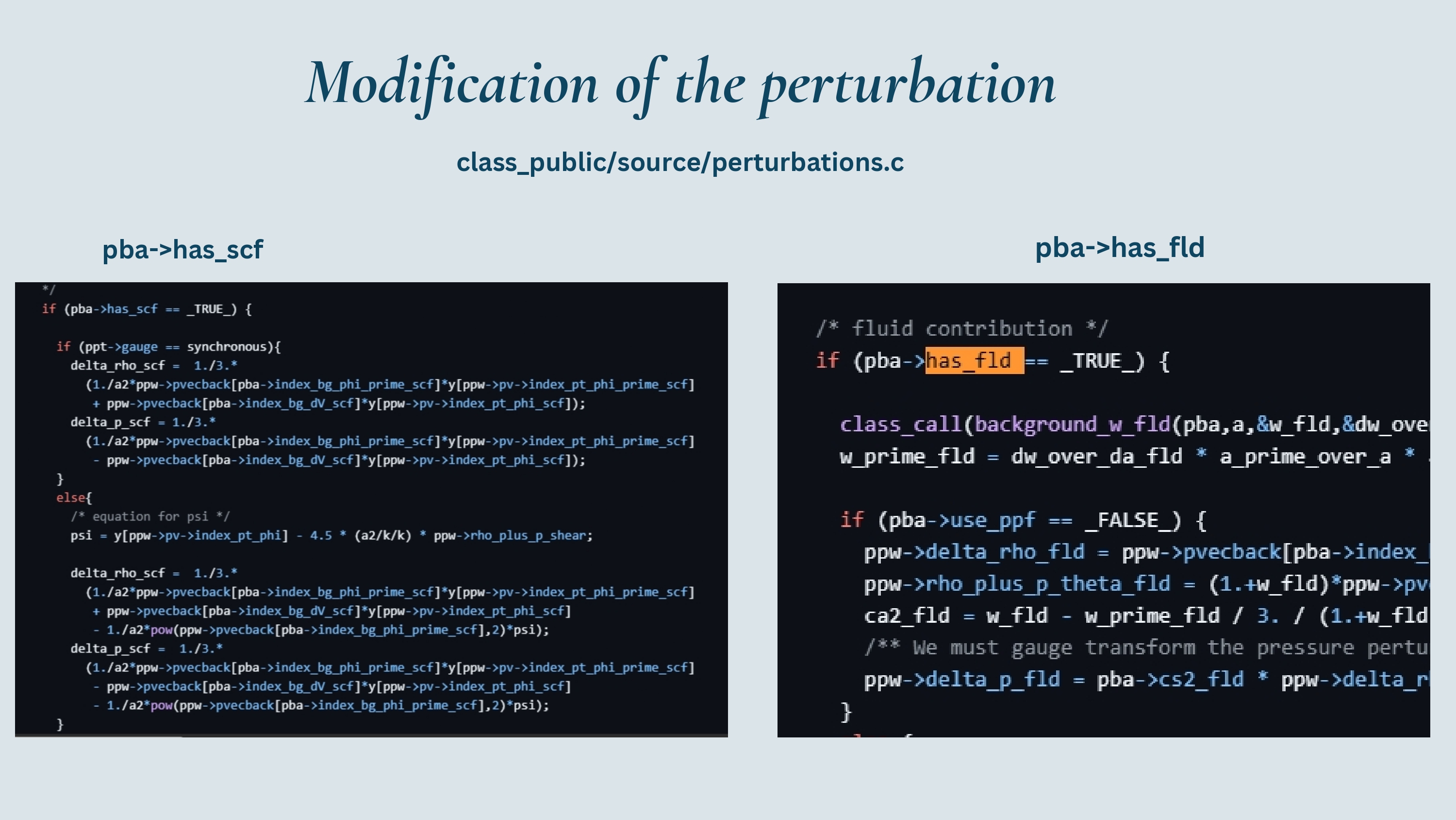
CLASS treats the perturbations of the scalar-field (scf) and fluid (fld) dark energy components separately. For phenomenological equation-of-state parameterizations such as CPL or JBP, the relevant part is the fluid perturbation sector, identified by has_fld.
Within this sector, CLASS again calls the background_w_fld() function to obtain the equation of state
and its derivative
\[\frac{dw_{\rm fld}}{da}.\]The derivative with respect to conformal time can then be obtained using
\[w_{\rm fld}' = \frac{dw_{\rm fld}}{da}\,a',\]where the prime denotes a derivative with respect to conformal time.
These quantities enter the evolution of the dark energy density, velocity, and pressure perturbations. For example, the adiabatic sound speed depends on both the equation of state and its time evolution and can be written schematically as
\[c_a^2 = w_{\rm fld} - \frac{w_{\rm fld}'} {3\mathcal{H}(1+w_{\rm fld})},\]where $\mathcal{H}=a’/a$ is the conformal Hubble parameter.
CLASS also allows the fluid rest-frame sound speed, represented by cs2_fld, to be specified independently. This quantity enters the calculation of the dark energy pressure perturbation.
For models in which $w(a)$ crosses the phantom divide $w=-1$, CLASS can employ the PPF (Parameterized Post-Friedmann) treatment through the use_ppf option, avoiding the singular behavior that can arise in the standard fluid perturbation equations near $1+w=0$.
Therefore, when implementing a new phenomenological dark energy parameterization, it is essential that the expression for $w_{\rm fld}(a)$ and its derivative $dw_{\rm fld}/da$ are defined consistently. Once these quantities are supplied through background_w_fld(), they can also be used by the perturbation module.
The figure below shows the separate scalar-field and fluid contributions implemented in perturbations.c, with the has_fld sector being the relevant one for the JBP implementation considered in this tutorial.
3. Implementing a New Dark Energy Model
Before modifying the CLASS source code, we first need to derive the quantities required by its fluid description. As an example, we consider the Jassal–Bagla–Padmanabhan (JBP) parameterization,
\[w(z)=w_0+w_1\frac{z}{(1+z)^2}.\]Using the relation
\[1+z=\frac{1}{a},\]we rewrite the equation of state in terms of the scale factor $a$. For the implementation in CLASS, we need to determine the equation of state $w(a)$, its derivative $dw/da$, and the corresponding dark energy density evolution function $f_{\rm DE}(a)$.
After performing these calculations, we obtain the JBP equation of state
\[w(a) = w_0 + w_1 a(1-a),\]its derivative
\[\frac{dw}{da} = w_1(1-2a),\]and the dark energy evolution function
\[f_{\mathrm{DE}}(a) = a^{-3(1+w_0)} \exp\left[\frac{3w_1}{2}(1-a)^2\right].\]The corresponding dark energy density is then
\[\rho_{\mathrm{DE}}(a) = \rho_{\mathrm{DE},0} f_{\mathrm{DE}}(a).\]These are the three main model-dependent quantities required to implement the JBP parameterization in the CLASS fluid description.
4. Modifying background.h
We are now ready to implement the JBP parameterization in CLASS. The first file that needs to be modified is
class_public/include/background.h
This file defines the available dark energy parameterizations and declares the variables used throughout the CLASS background module. Therefore, before implementing the JBP equations, we must first register the new model and define its corresponding parameters.
Step 1: Register the JBP Parameterization
Locate the following line in background.h:
enum equation_of_state {CLP,EDE};
and add the JBP parameterization:
enum equation_of_state {CLP,EDE,JBP};
This informs CLASS that a new fluid equation-of-state parameterization named JBP is available.
Step 2: Define the JBP Parameters
Next, locate the fluid equation-of-state parameters
double w0_fld; /**< \f$ w0_{DE} \f$: current fluid equation of state parameter */
double wa_fld; /**< \f$ wa_{DE} \f$: fluid equation of state parameter derivative */
Immediately below these lines, add the two parameters of the JBP model:
double w0_jbp;
double w1_jbp;
Here,
w0_jbpis the present-day value of the dark energy equation of state.w1_jbpcontrols the time evolution of the equation of state.
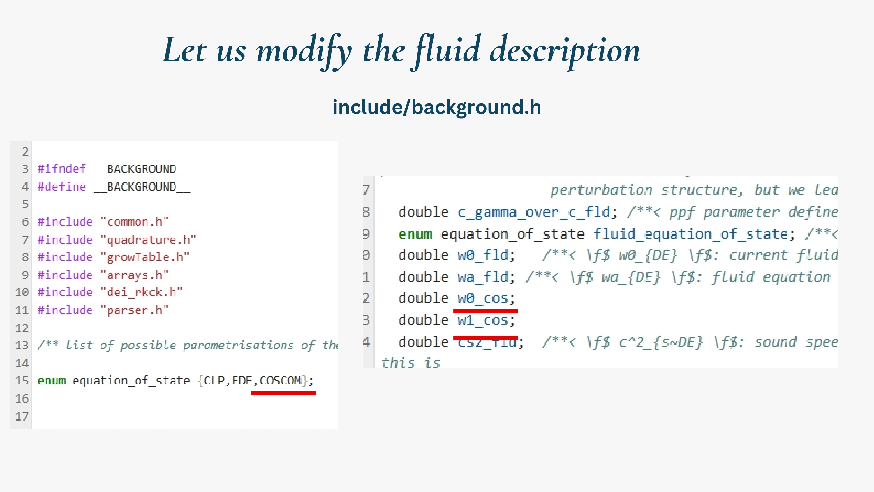
The figure below highlights the required modifications in background.h.
5. Modifying background.c
The next step is to implement the JBP parameterization in the CLASS background evolution. All modifications are performed in
class_public/source/background.c
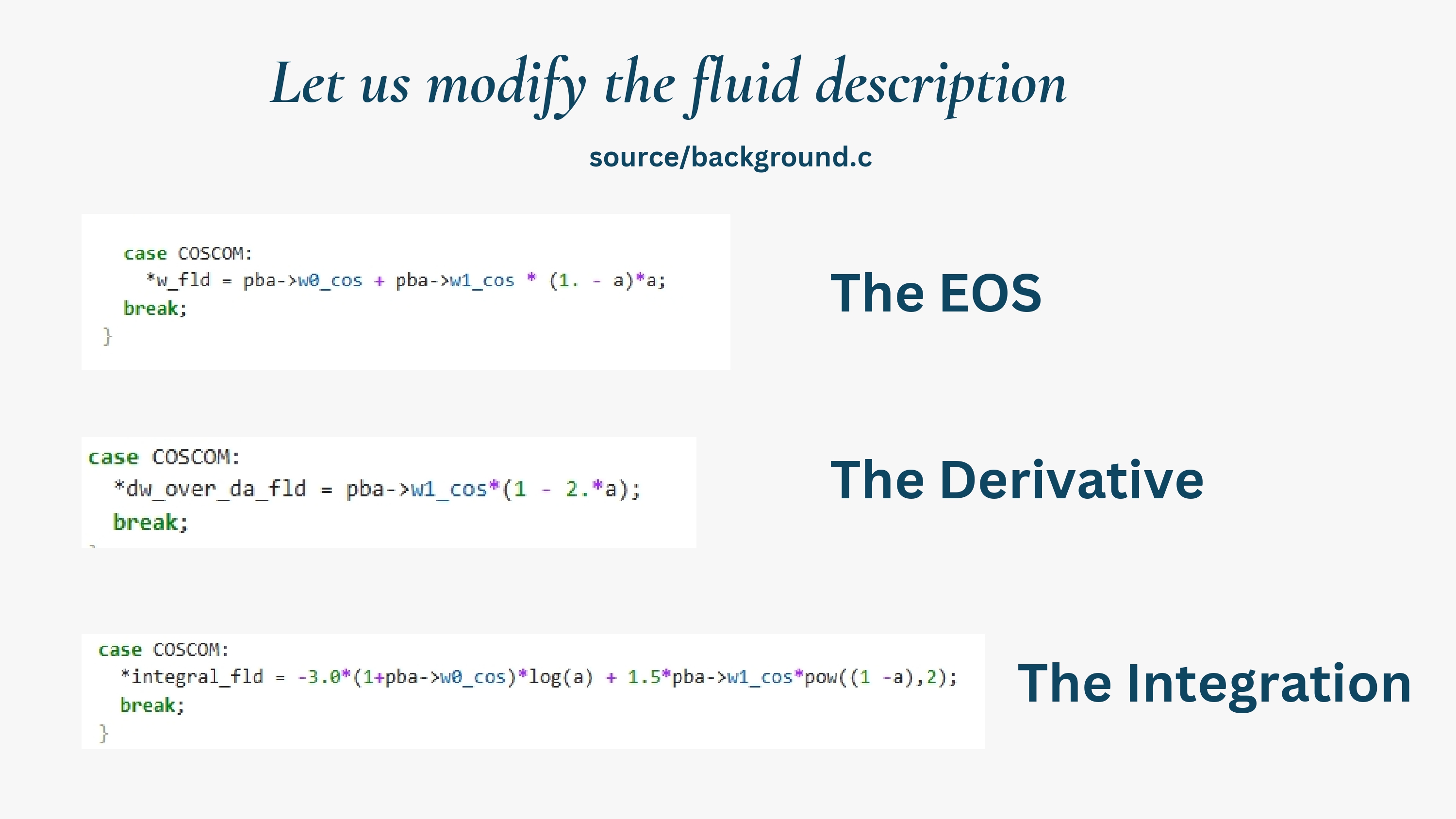
The function background_w_fld() is responsible for computing the fluid equation of state, its derivative, and the integral that determines the dark energy density evolution. Therefore, we need to add a new JBP case in each of these three sections.
Step 1: Define the JBP Equation of State
Locate the switch statement that computes the fluid equation of state,
switch (pba->fluid_equation_of_state) {
case CLP:
  *w_fld = pba->w0_fld + pba->wa_fld * (1. - a);
  break;
}
and add the JBP implementation:
case JBP:
  *w_fld = pba->w0_jbp + pba->w1_jbp * a * (1. - a);
  break;
This implements the JBP equation of state
\[w(a)=w_0+w_1a(1-a).\]Step 2: Define the Derivative
Next, locate the switch statement that computes the derivative of the equation of state,
switch (pba->fluid_equation_of_state) {
case CLP:
  *dw_over_da_fld = -pba->wa_fld;
  break;
}
and add
case JBP:
  *dw_over_da_fld = pba->w1_jbp * (1. - 2.*a);
  break;
This corresponds to
\[\frac{dw(a)}{da}=w_1(1-2a).\]Step 3: Define the Dark Energy Density Evolution
Finally, locate the switch statement that computes the integral controlling the evolution of the dark energy density,
switch (pba->fluid_equation_of_state) {
case CLP:
  *integral_fld =
      3.*((1.+pba->w0_fld+pba->wa_fld)*log(1./a)
      + pba->wa_fld*(a-1.));
  break;
}
and add
case JBP:
  *integral_fld =
      -3.*(1.+pba->w0_jbp)*log(a)
      + 1.5*pba->w1_jbp*pow(1.-a,2.);
  break;
This implements the JBP dark energy evolution function
\[f_{\mathrm{DE}}(a) = a^{-3(1+w_0)} \exp\left[ \frac{3w_1}{2}(1-a)^2 \right].\]Once these three modifications are completed, the CLASS background module will be able to compute the JBP equation of state, its derivative, and the corresponding dark energy density evolution.
6. Modifying input.c
The next file that must be modified is
class_public/source/input.c
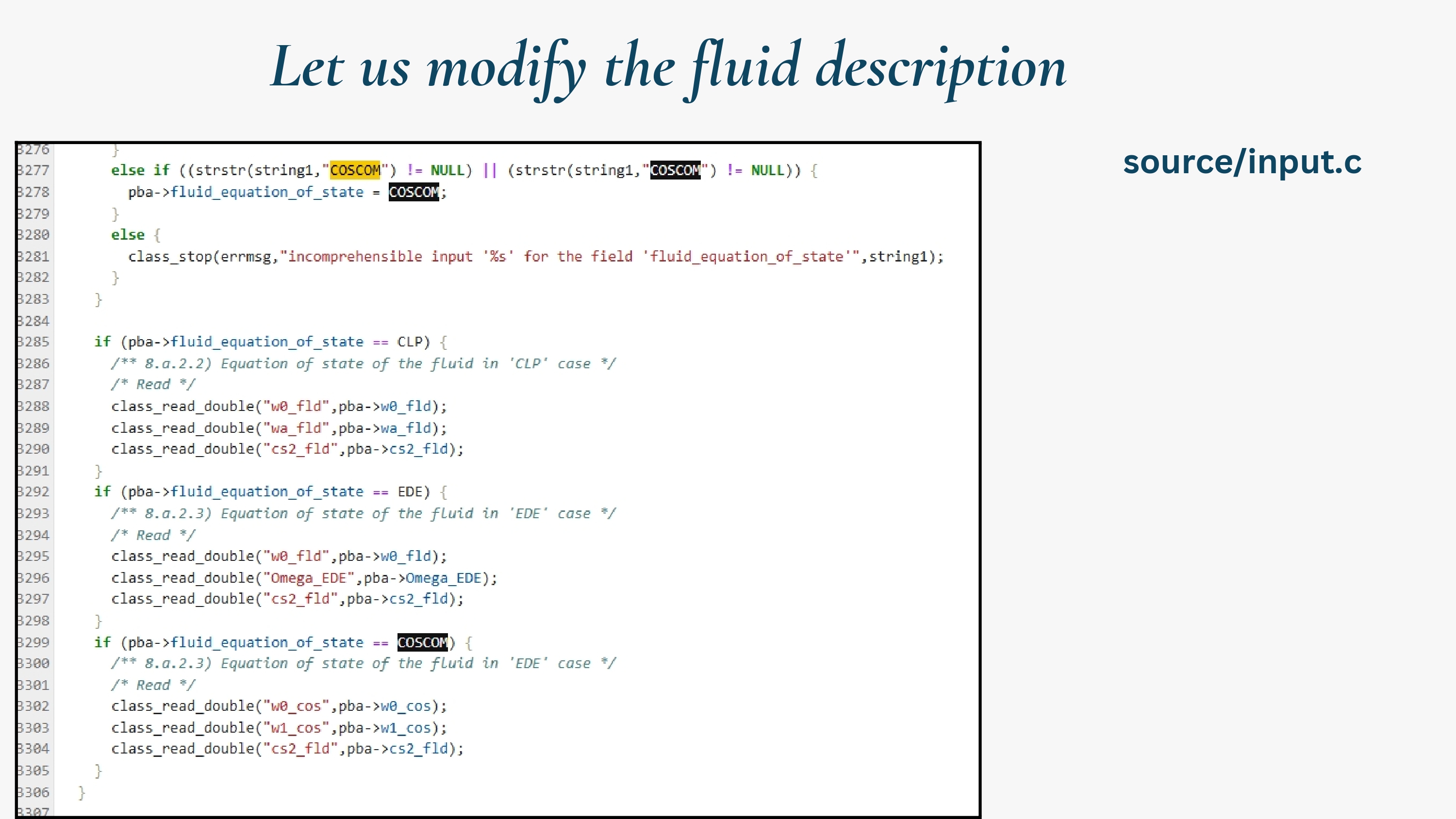
This file is responsible for reading the cosmological parameters supplied by the user and initializing their default values. To support the JBP parameterization, we need to perform two modifications.
Step 1: Read the JBP Parameters
Locate the section where CLASS reads the fluid equation-of-state parameterization and its corresponding parameters. Extend the existing implementation by adding a new JBP case.
First, register the new equation-of-state parameterization:
/* Complete set of parameters */
if (flag1 == _TRUE_) {

  if ((strstr(string1,"CLP") != NULL) ||
      (strstr(string1,"clp") != NULL)) {
    pba->fluid_equation_of_state = CLP;
  }

  else if ((strstr(string1,"JBP") != NULL) ||
           (strstr(string1,"jbp") != NULL)) {
    pba->fluid_equation_of_state = JBP;
  }
}
Next, instruct CLASS to read the JBP model parameters from the input file:
if (pba->fluid_equation_of_state == CLP) {

  class_read_double("w0_fld", pba->w0_fld);
  class_read_double("wa_fld", pba->wa_fld);
  class_read_double("cs2_fld", pba->cs2_fld);

}

if (pba->fluid_equation_of_state == JBP) {

  class_read_double("w0_jbp", pba->w0_jbp);
  class_read_double("w1_jbp", pba->w1_jbp);
  class_read_double("cs2_fld", pba->cs2_fld);

}
This modification allows CLASS to recognize the keyword JBP and read the corresponding model parameters from the input configuration file.
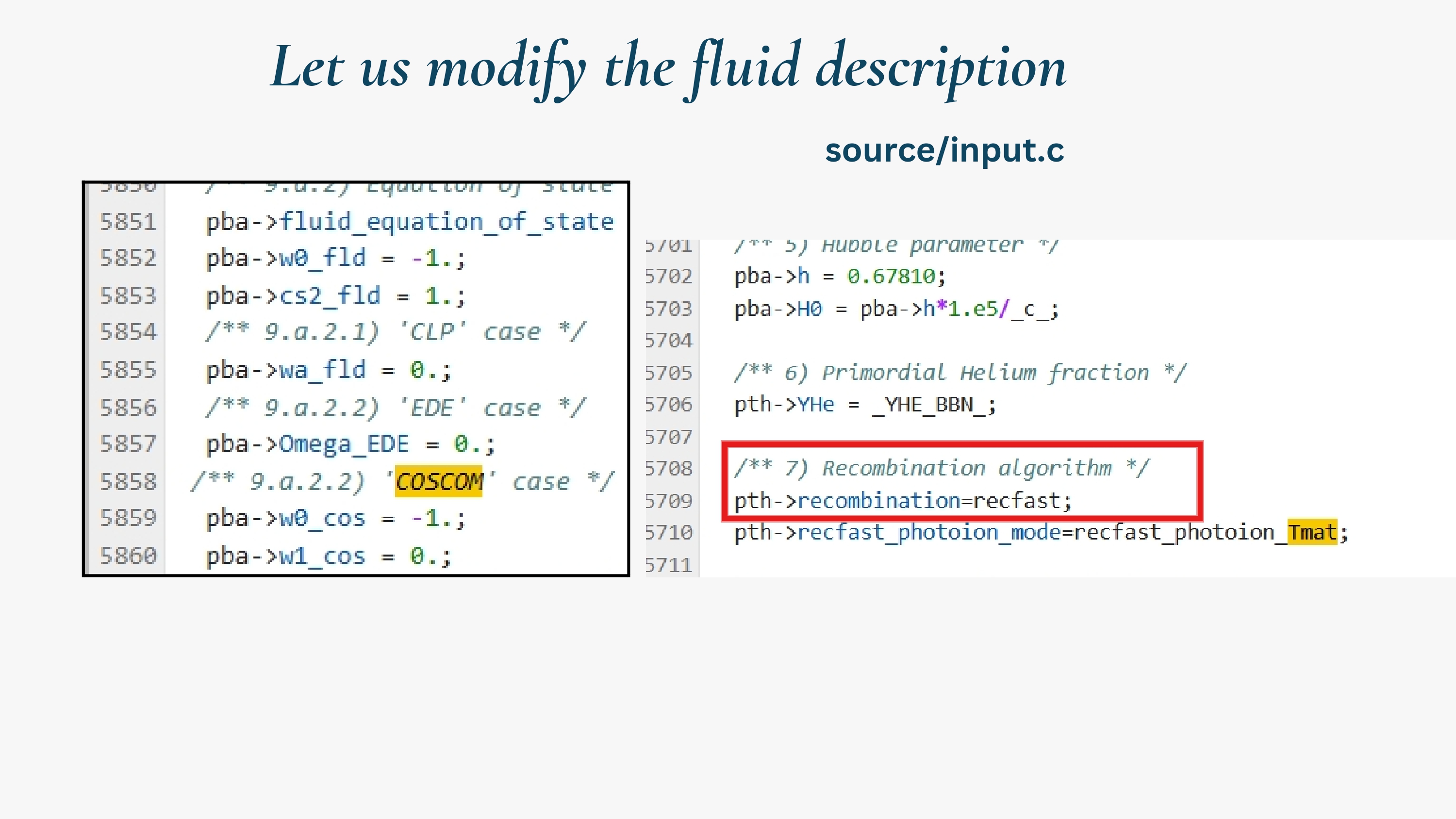
Step 2: Initialize the Default Values
Further down in the same file, locate the section where the default values of the fluid parameters are initialized.
The standard CLASS implementation contains
pba->fluid_equation_of_state = CLP;

pba->w0_fld = -1.;
pba->wa_fld = 0.;
pba->cs2_fld = 1.;
Immediately below these lines, add the default values for the JBP parameters:
/** JBP default parameters */

pba->w0_jbp = -1.;
pba->w1_jbp = 0.;
These default values ensure that all newly introduced variables are properly initialized before being overwritten by the values provided in the input file.
Once these two modifications have been completed, CLASS can successfully recognize the JBP parameterization and read its free parameters from the input configuration.
7. Updating the Python Interface
The final modification is to expose the newly added JBP parameters to the Python interface. This step is required if you plan to use MontePython, Cobaya, or directly access the parameters through the CLASS Python wrapper.
Open
class_public/python/classy.pxd
and add the same variables that were introduced in background.h.
double w0_fld
double wa_fld

double w0_jbp
double wa_jbp
By adding these declarations, the Python wrapper is informed that these variables exist inside the CLASS background structure, making them accessible from Python-based cosmological analysis codes.
After this modification, the new JBP parameters are fully connected throughout CLASS, from the C source code to the Python interface.